Introduction to Local Functions

The Local functions of LCZ4r are specialized tools designed to analyze large datasets, such as hourly air temperature readings. This tutorial focuses on using data from Berlin, collected across 23 meteorological stations as part of the Urban Climate Observatory (UCO)

Overview

The Local functions in LCZ4r, offer powerful tools to handle and analyze urban climate data. They enable time-series analysis, mapping of thermal anomalies, spatial interpolation, and more. Below is a summary of these functions:

Function	Description	Data Required	Internet Access Required
`lcz_ts()`	Analyze LCZ Time Series	Yes	Optional
`lcz_anamoly()`	Calculate LCZ Thermal Anomalies	Yes	Optional
`lcz_anamoly_map()`	Map LCZ Thermal Anomalies	Yes	Optional
`lcz_interp_map()`	Perform LCZ Interpolation	Yes	Optional
`lcz_plot_interp()`	Visualize LCZ Interpolation	Yes	Optional
`lcz_uhi_intensity()`	Assess LCZ for Urban Heat Island Intensity	Yes	Optional

💡 Tips:

Utilize the help(lcz_*) function to access detailed documentation for each LCZ4r function. For example, to learn about the lcz_ts function, type help(“lcz_ts”) in the console.
Each LCZ4r function supports imputation for handling missing values within data frames. For more information on imputation methods, refer to the “impute” argument in the documentation of each function.

Data input requirements

To ensure smooth operation of the local functions, input data should be structured as a data frame with the following columns:

date: This column should contain date-time information. This column must labeled “date”.
Station Identifier: A column for identifying meteorological stations.
Air Temperature or other variable: At least one column representing the air temperature or any other target variable.
Latitude and Longitude: Two columns for the geographical coordinates of each station.

Ensure that the date-time format aligns with R’s conventions (e.g., YYYY-MM-DD HH:MM:SS). Acceptable formats include “1/2/1999” or “1999-02-01”

To simplify this setup, LCZ4r provides a sample data frame, which you can load with the following command:

library(LCZ4r)

#Load data from LCZ4r package
data("lcz_data")

#Check data structure out
str(lcz_data)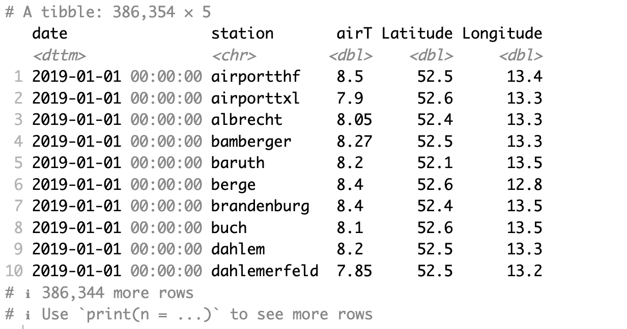

Import your data

if(!require(data.table)) install.packages("data.table")

library(data.table)

#Load data from your PC
my_data <- fread("PC/path/file_name.csv")

#Check data structure out
str(my_data)

Customizing Local Functions in LCZ4r

You can further customize the Local Functions to suit specific analysis needs:

1. Flexibility time selection

The Local Functions have an argument … that provides options to filter data by specific years, months, days, and hours to narrow down your analysis period. Examples of how to use these arguments include:

Year(s): Numeric value(s) specifying the year(s) to select. For example, year = 1998:2004 selects all years between 1998 and 2004 (inclusive), while year = c(1998, 2004) selects only the years 1998 and 2004.
Month(s): Numeric or character value(s) specifying the months to select. Numeric examples: month = 1:6 (January to June), or character examples: month = c(“January”, “December”).
Day(s): Numeric value(s) specifying the days to select. For instance, day = 1:30 selects days from 1 to 30, or day = 15 selects only the 15th day of the month.
Hour(s): Numeric value(s) specifying the hours to select. For example, hour = 0:23 selects all hours in a day, while hour = 9 selects only the 9th hour.
Start date: A string specifying the start date in either start=“DD/MM/YYYY” (e.g., “1/2/1999”) or “YYYY-mm-dd” format (e.g., “1999-02-01”).
End date: A string specifying the end date in either end=“DD/MM/YYYY” (e.g., “1/2/1999”) or “YYYY-mm-dd” format (e.g., “1999-02-01”).

Examples

#Select a range of years (e.g., 1998:2004) or specific years (e.g., c(1998, 2004)).
lcz_ts(
  lcz_map,
  year=1998:2004
)

#Filter by month, either by numeric values (e.g., 1:6 for January to June) or by names (e.g., c("January", "December")).
lcz_anomlay(
  lcz_map,
  year=2012, month=9
)

# Pinpoint a specific date, such as September 1, 2019, by setting the *year*, *month*, *day*, as arguments.
lcz_interp_map(
  lcz_map,
  year=2012, month=9, day=1 
)
# For a specific hour.
lcz_interp_map_anomaly(
  lcz_map,
  year=2012, month=9, day=1, hour=5
)

#Pinpoint a specific period, by setting *start*=1/9/1986 and *end*=1/9/2024, as arguments.
lcz_uhi_intensity(
  lcz_map,
  var = "airT", 
  station_id = "station",
  start="1/9/2019", end="30/10/2019"
)

For more information, see the utility functions from the openair package.

2. Splitting LCZ time series by temporal window or site

You can segment the LCZ time series data using the by argument, allowing for analysis across different temporal windows or sites. Available split options include:

1. Temporal segments: “year”, “season”, “seasonyear”, “month”, “monthyear”, “weekday”, “weekend”.
1. Daylight split: “daylight”, which divides data into daytime and nighttime periods.
1. You can use also c(“daylight”, “month”), c(“daylight”, ““season”)

For further details, refer to the type in openair package:

Have feedback or suggestions?

Do you have an idea for improvement or did you spot a mistake? We’d love to hear from you! Click the button below to create a new issue (Github) and share your feedback or suggestions directly with us.

Max Anjos