Temperature Modeling with LCZ

Introduction

Understanding temperature variations within urban environments is very important for climate research, particularly when examining Urban Heat Islands. The LCZ4r package offers functions for creating interpolated maps and thermal anomaly analyses within Local Climate Zones (LCZs). lcz_interp_map() or lcz_anomaly_mapfunctions can be applied to generate detailed spatial representations of air temperature, allowing researchers to analyze the influence of urban structures and land use on local climates.

In this guide, we’ll demonstrate how to use the lcz_interp_map() or lcz_anomaly_mapfunctions to model temperature data across Berlin’s LCZ. This will involve creating maps at specific times, customizing spatial and temporal resolutions, and visualizing thermal anomalies.

Modelling climate with LCZ

The lcz_interp_map() or lcz_anomaly_map() functions are used to generate a map of interpolated air temperatures. These functions apply interpolation techniques, like the Kriging model, to estimate air temperatures based on LCZ classes, enabling a spatially-resolved understanding of temperature variations. The parameters for time frequency and data segmentation are consistent with those used in lcz_ts() and lcz_anomaly(), but two additional arguments are introduced:

sp.res: Specifies the spatial resolution of the output map in meters. Default is 100
tp.res: Defines the time frequency at which values are averaged. Default is hour

The lcz_interp_map() and lcz_anomaly_map() functions generate either a single raster file or a stack of rasters. You can visualize the resulting interpolated map using the lcz_plot_interp() function, creating a clear representation of air temperature distributions across the selected LCZs.

# Get the LCZ map for your city
lcz_map <- lcz_get_map_euro(city="Berlin")

# Load sample data from LCZ4r
data("lcz_data")

Interpolating air temperature with LCZ

Single hour map interpolation

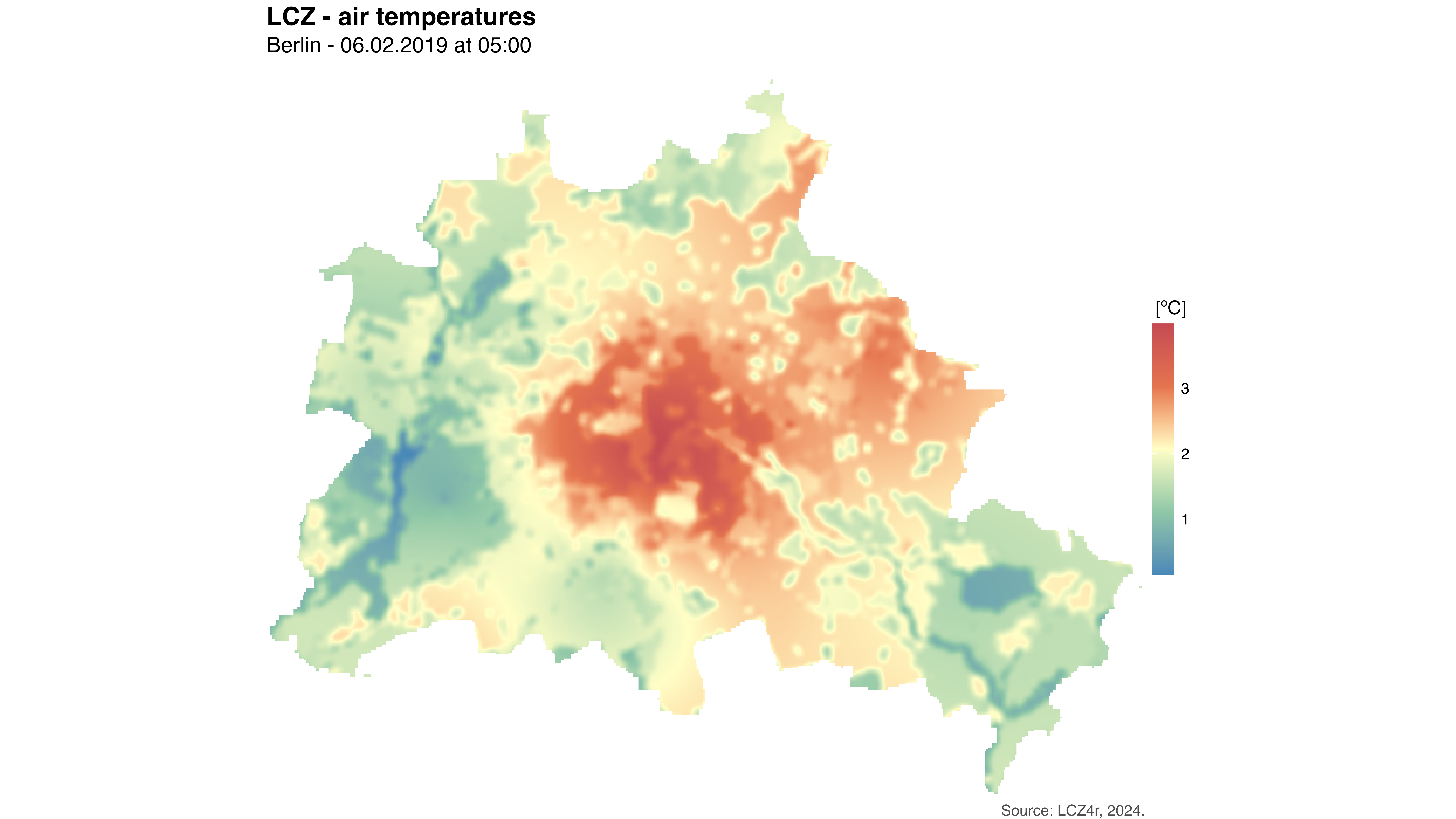
The following example demonstrates how to generate a temperature map for a specific date and time.


#Mapping air temperatures for 6th February 2019 at 05:00h 
my_interp_map <- lcz_interp_map(lcz_map,
                                data_frame = lcz_data, 
                                var = "airT", station_id = "station",
                                sp.res = 100, tp.res = "hour",
                                 year = 2019, month = 2, day = 6, hour = 5)

#Customize the plot with titles and labels
lcz_plot_interp(my_interp_map, 
                title = "LCZ - air temperatures", 
                subtitle = "Berlin - 06.02.2019 at 05:00",
                caption = "Source: LCZ4r, 2024.",
                fill = "[ºC]")

Hourly Interpolation Over a Day

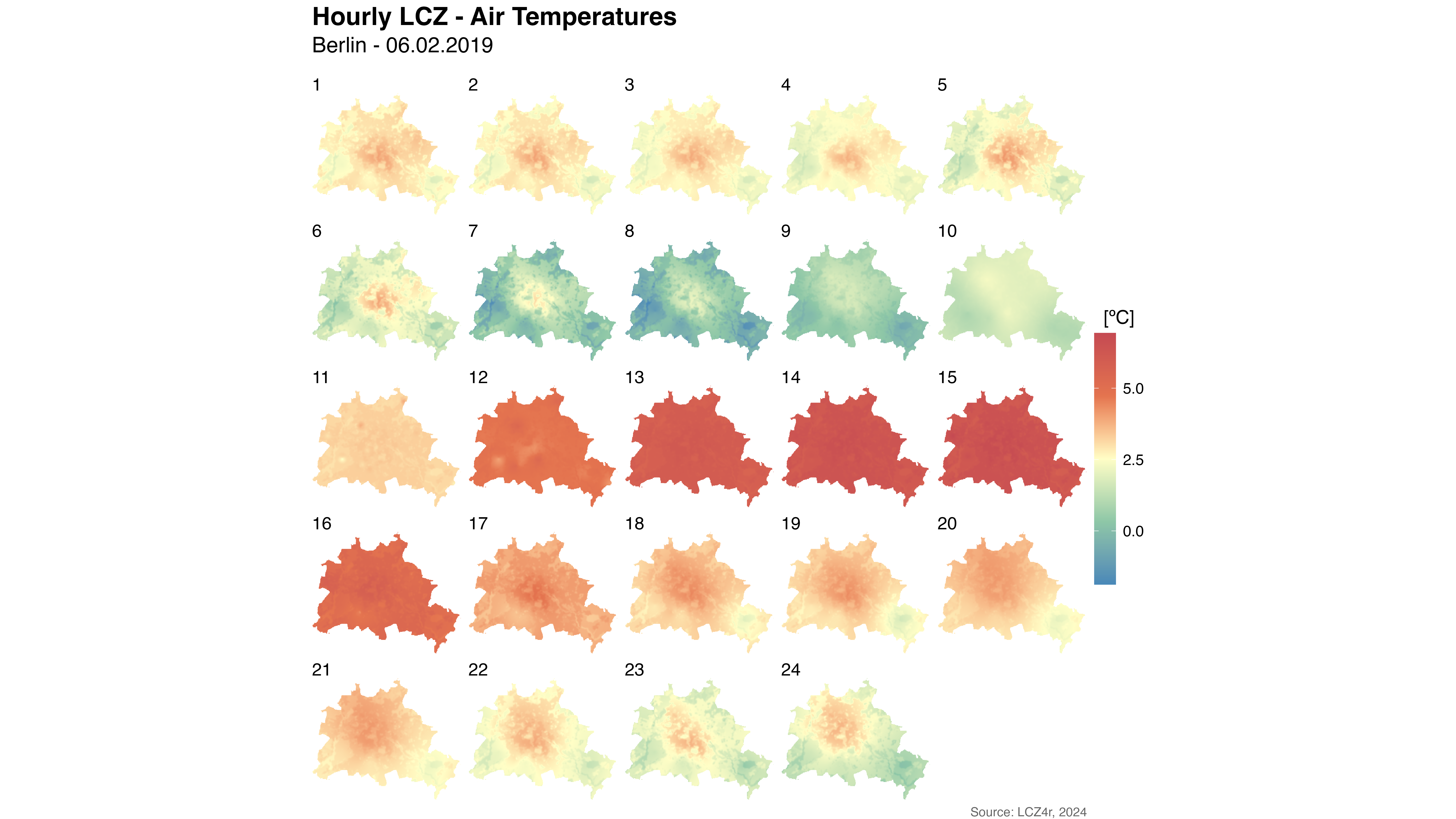
The by argument allows you to generate a sequence of hourly temperature maps for a specific day. Here, each hour will be represented by an individual raster layer.


# Active the by argument! Mapping air temperature for each hour
my_interp_map <- lcz_interp_map(lcz_map,
                                data_frame = lcz_data, 
                                var = "airT", station_id = "station",
                                sp.res = 100, tp.res = "hour",
                                year = 2019, month = 2, day = 6,
                                by = "hour")

#Rename raster names with hour
names(my_interp_map) <- c(1:24)

lcz_plot_interp(my_interp_map, 
                title = "Hourly LCZ - air temperatures", 
                subtitle = "Berlin - 06.02.2019",
                caption = "Source: LCZ4r, 2024.",
                fill = "[ºC]")

Interpolating thermal anomalies with LCZ

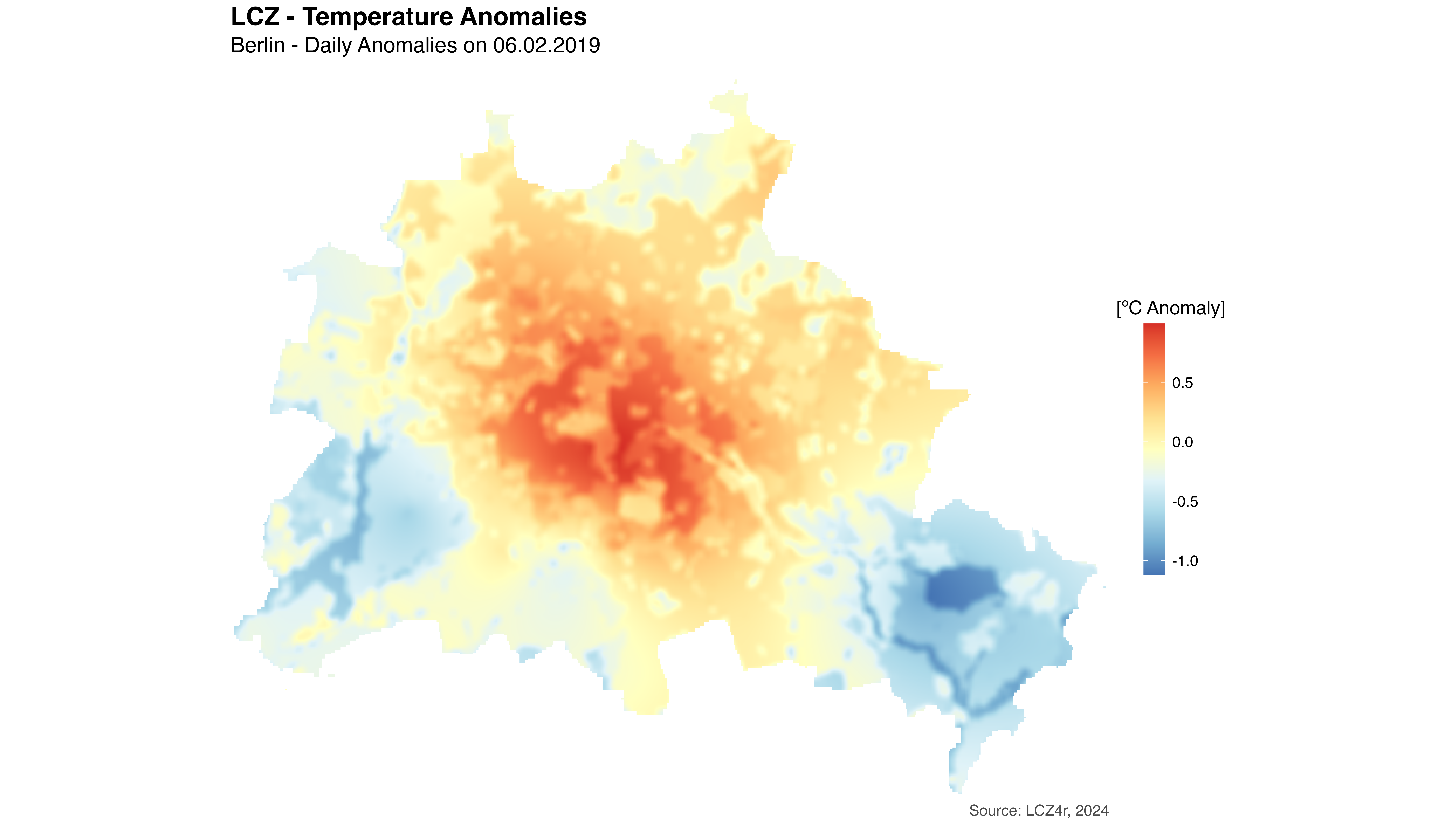
The lcz_anomaly_map() function can be used to highlight temperature anomalies relative to the average conditions across LCZs. Anomaly maps are useful in identifying areas where temperatures significantly differ from typical values, such as heat hotspots within urban areas.

Single day map interpolation


# Generate an anomaly map for a specified day
my_anomaly_map <- lcz_anomaly_map(lcz_map,
                                  data_frame = lcz_data,
                                  var = "airT", station_id = "station",
                                  sp.res = 100, tp.res = "day",
                                  year = 2019, month = 2, day = 6)

# Plotting the thermal anomaly map
lcz_plot_interp(my_anomaly_map,
                title = "LCZ - Temperature Anomalies",
                subtitle = "Berlin - Daily Anomalies on 06.02.2019",
                caption = "Source: LCZ4r, 2024",
                fill = "[ºC Anomaly]",
                palette = "bl_yl_rd"
                )

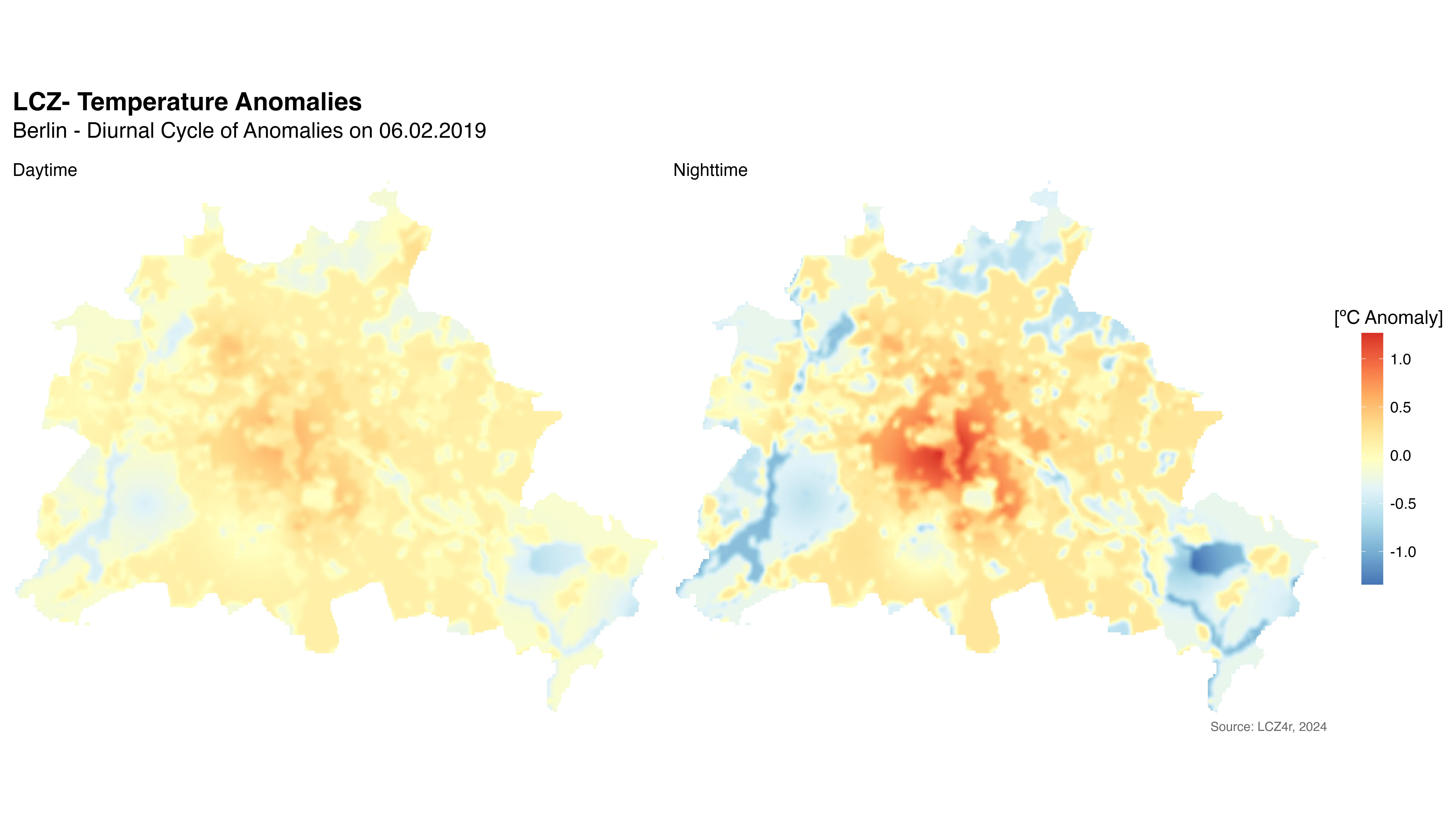
Daytime and nighttime anomalies


# Split up anomalies into daytime and nighttime with by="daylight" 
my_anomaly_map <- lcz_anomaly_map(lcz_map,
                                  data_frame = lcz_data,
                                  var = "airT", station_id = "station",
                                  sp.res = 100, tp.res = "hour",
                                  year = 2019, month = 2, day = 6,
                                  by = "daylight")
#Rename raster
names(my_anomaly_map) <- c("Daytime", "Nighttime")

# Plotting the thermal anomaly map
lcz_plot_interp(my_anomaly_map,
                title = "LCZ- Temperature Anomalies",
                subtitle = "Berlin - Diurnal Cycle of Anomalies on 06.02.2019",
                caption = "Source: LCZ4r, 2024",
                fill = "[ºC Anomaly]",
                palette = "bl_yl_rd",
                )

Have feedback or suggestions?

Do you have an idea for improvement or did you spot a mistake? We’d love to hear from you! Click the button below to create a new issue (Github) and share your feedback or suggestions directly with us.

Max Anjos

November 19, 2024