Time Series Analysis

Getting Started

The lcz_ts() function allows you to analyze air temperature data associated with Local Climate Zones (LCZ) over time. In this tutorial, we’ll perform an hourly frequency analysis of air temperature in Berlin for the years 2019-2020 using lcz_data from the LCZ4r package.

# Get the LCZ map for your city
lcz_map <- lcz_get_map_euro(city="Berlin")

# Load sample data from LCZ4r
data("lcz_data")

Basic Time Series Analysis

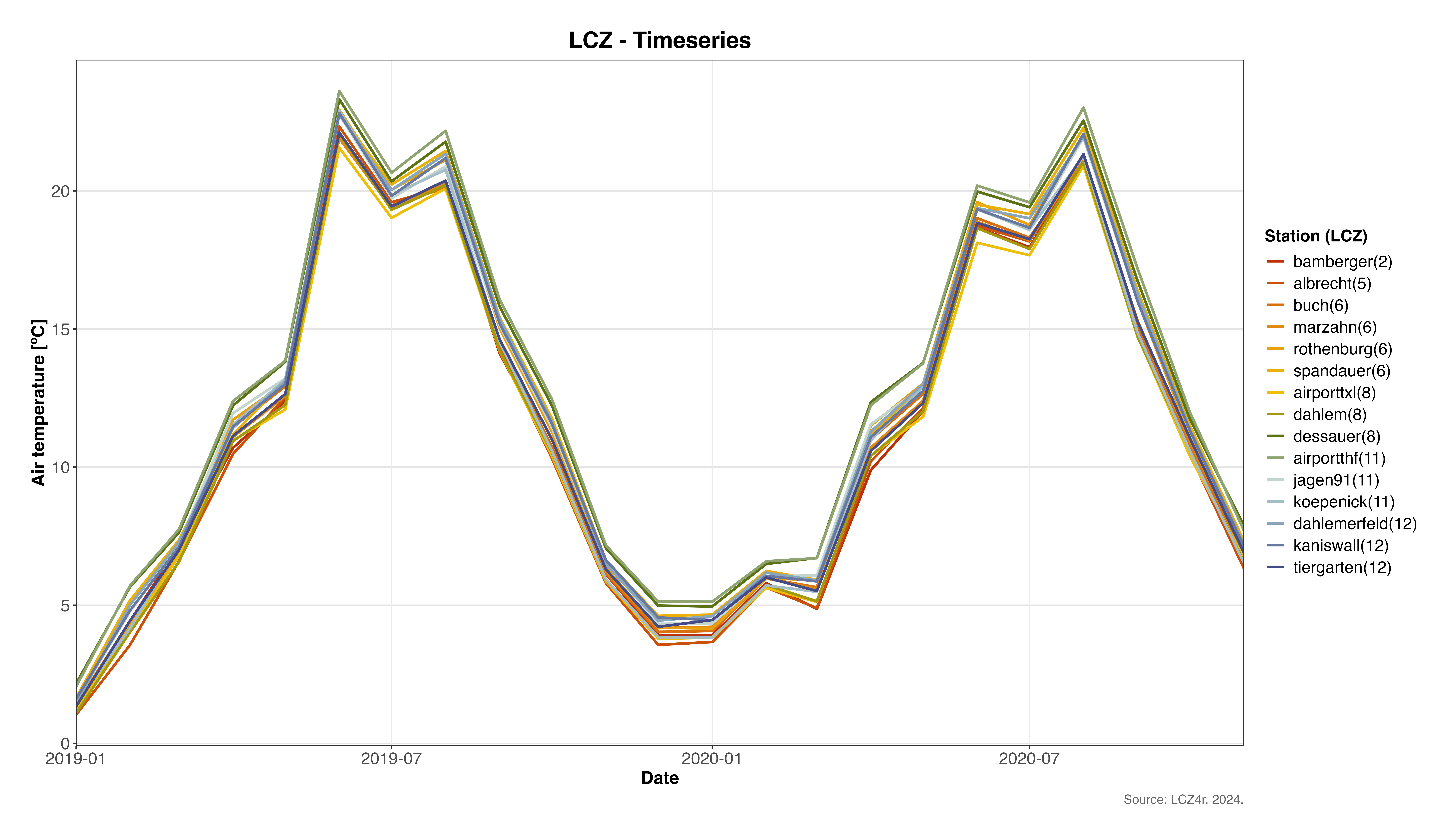
Let’s start with a basic analysis using lcz_ts() to observe hourly temperature fluctuations.


#Let's get monthly LCZ-air temperature time series
lcz_ts(lcz_map, 
       data_frame = lcz_data, 
       var = "airT", 
       station_id = "station",
       time.freq = "month",
       ylab = "Air temperature [ºC]",
       xlab = "Date",
       title = "LCZ - Timeseries",
       caption = "Source: LCZ4r, 2024."
       )

Plotting Options with plot_type

The plot_type argument in lcz_ts() offers several visualizations:

“basic_line”: Simple line plot
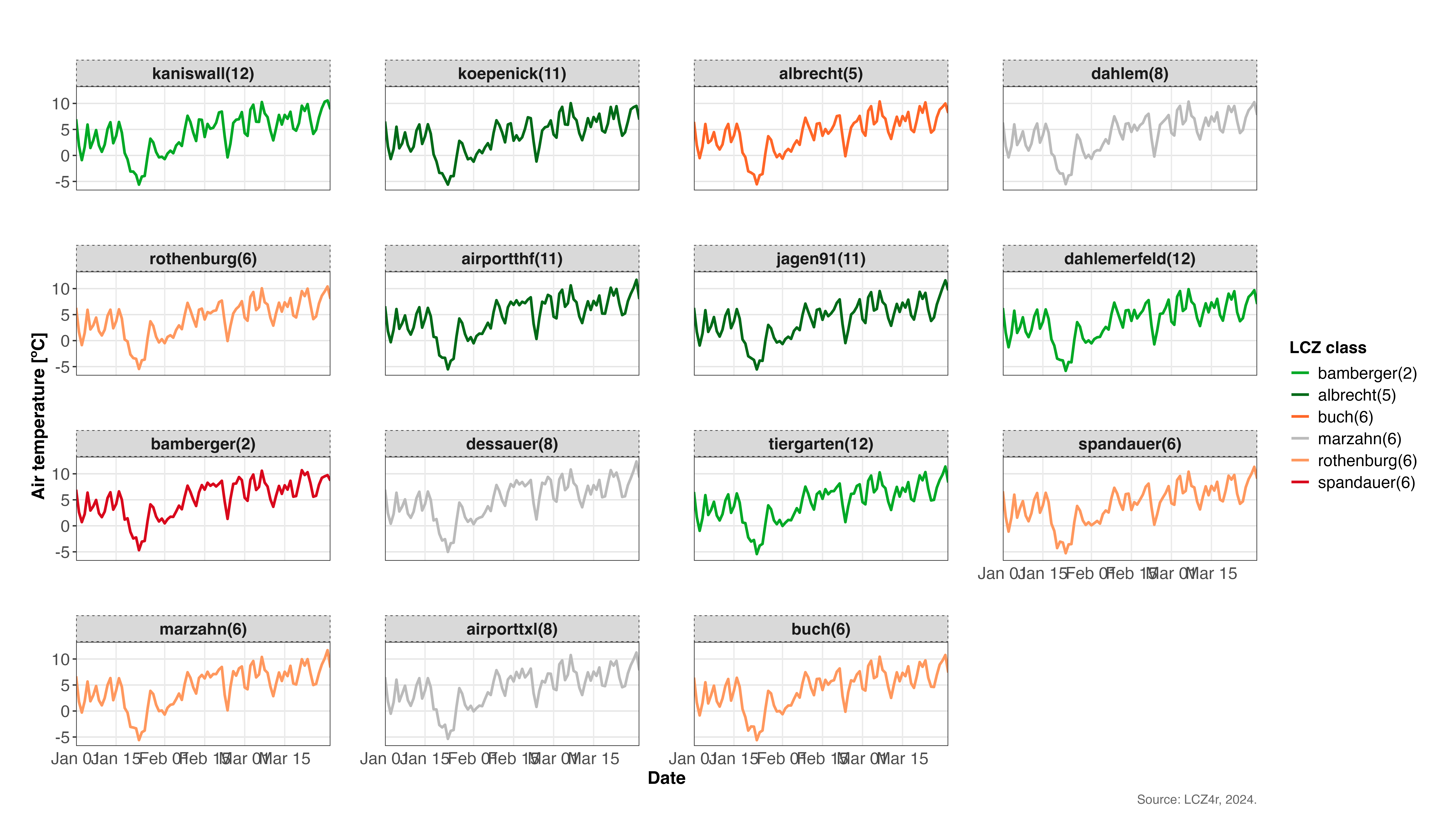
“faceted_line”: Line plot with facets by LCZ or station
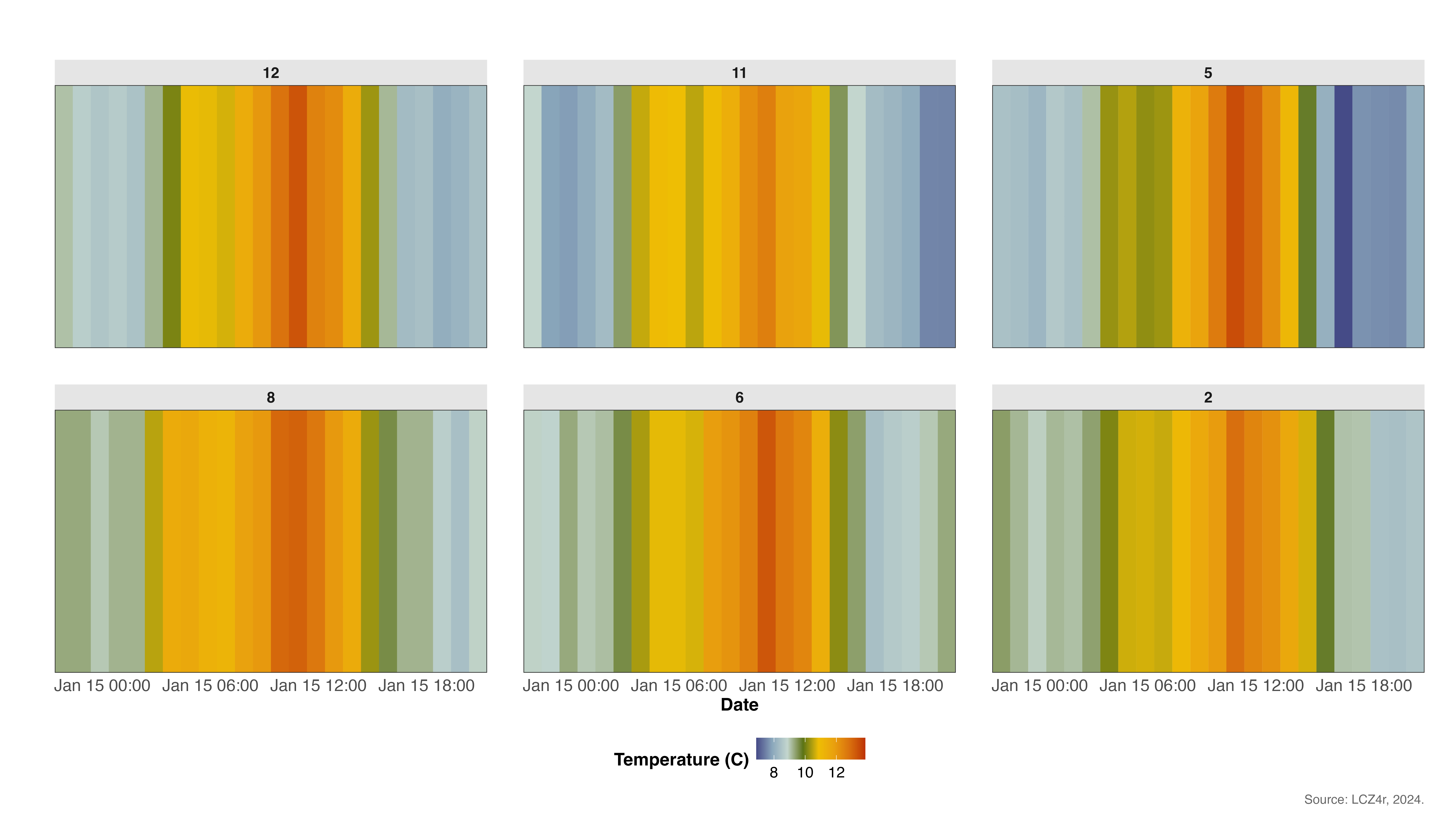
“heatmap”: Heatmap to visualize temporal patterns
“warming_stripes”: Stripes representing temperature variations over time Below are examples using each plot type.

1. Basic Line Plot


#Daily air temperature for September of 2019,
lcz_ts(lcz_map, 
       data_frame = lcz_data, 
       var = "airT", 
       station_id = "station",
       time.freq = "day",
       year = 2019, month=9,
       plot_type = "basic_line")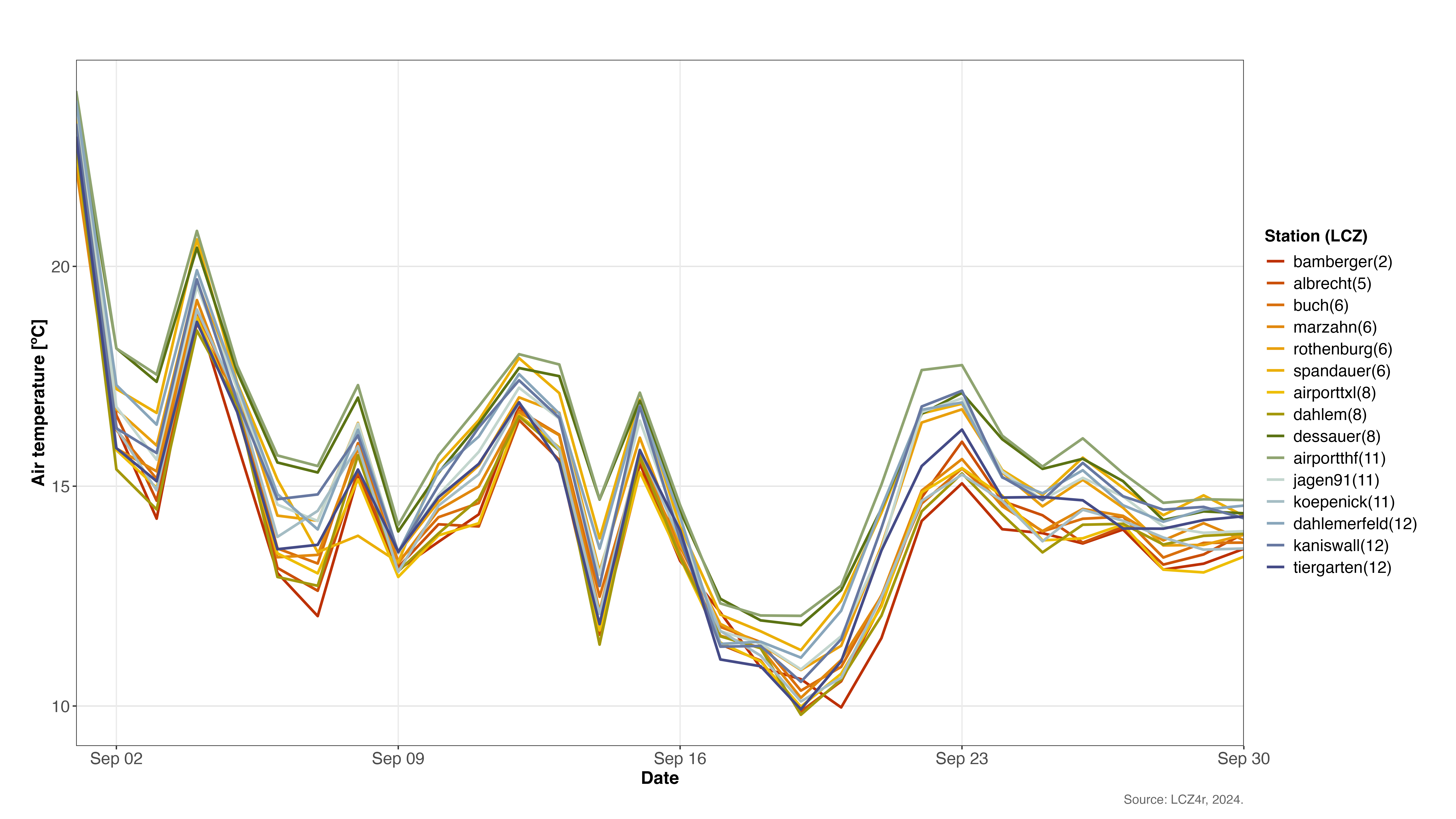

2. Faceted Line Plot by Station

#Daily air temperature from January and March of 2019 
lcz_ts(lcz_map, data_frame = lcz_data, var = "airT", 
       station_id = "station", time.freq = "hour",
       year = 2019, month=1:3,
       plot_type = "facet_line", 
       facet="station"
       )

3. Heatmap of Temperature Over Time

#Hourly air temperature on 15th January of 2020
lcz_ts(lcz_map, data_frame = lcz_data, var = "airT", 
       station_id = "station", time.freq = "hour",
       year = 2020, month=1, day=15,
       plot_type = "heatmap", 
       facet="LCZ"
       )

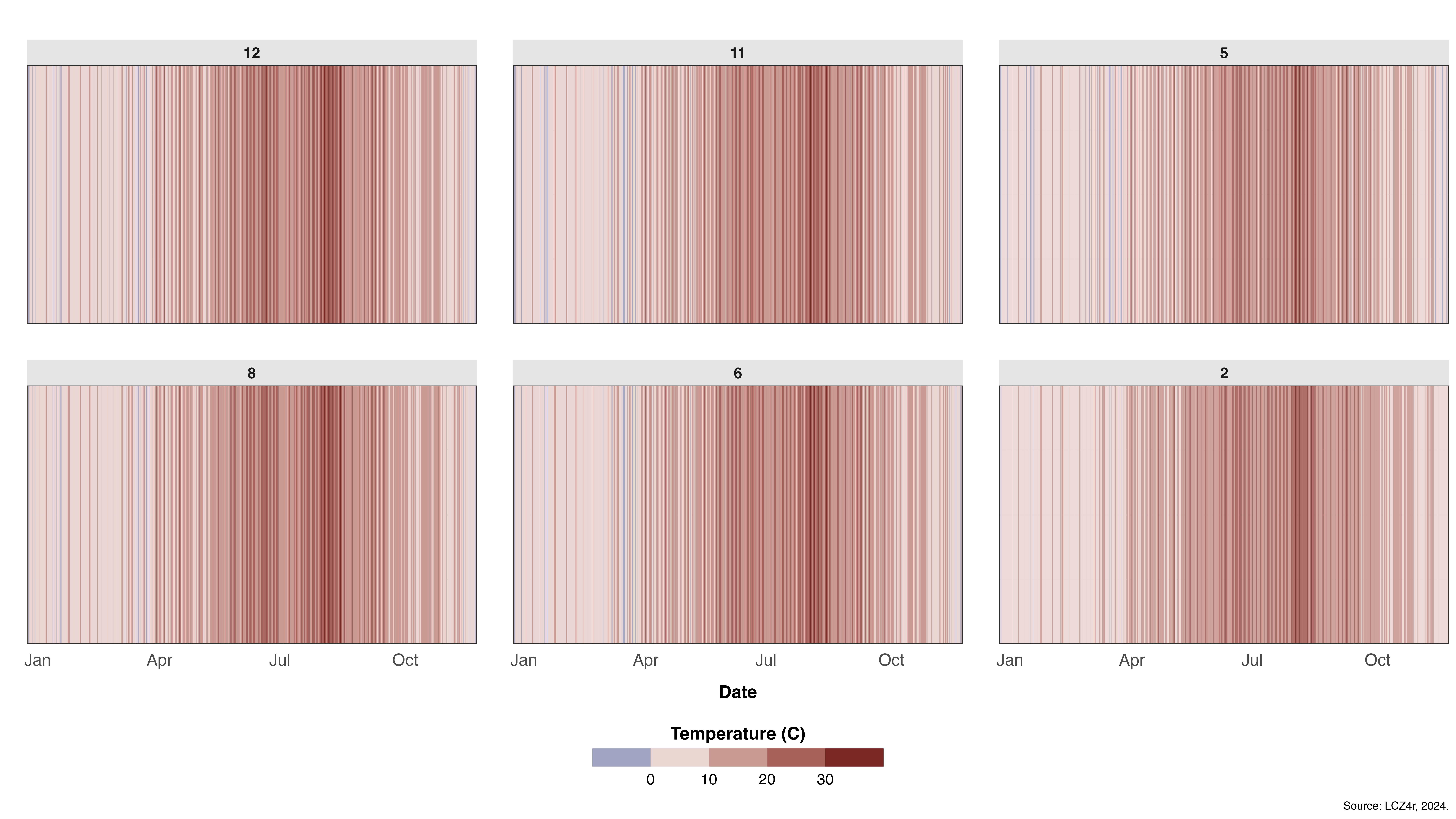
4. Warming Stripes


#Hourly air temperature for 2020
lcz_ts(lcz_map, data_frame = lcz_data, var = "airT", 
       station_id = "station", time.freq = "hour", 
       year = 2012, month = 1:12,
       plot_type = "warming_stripes",
       facet="LCZ"
       )

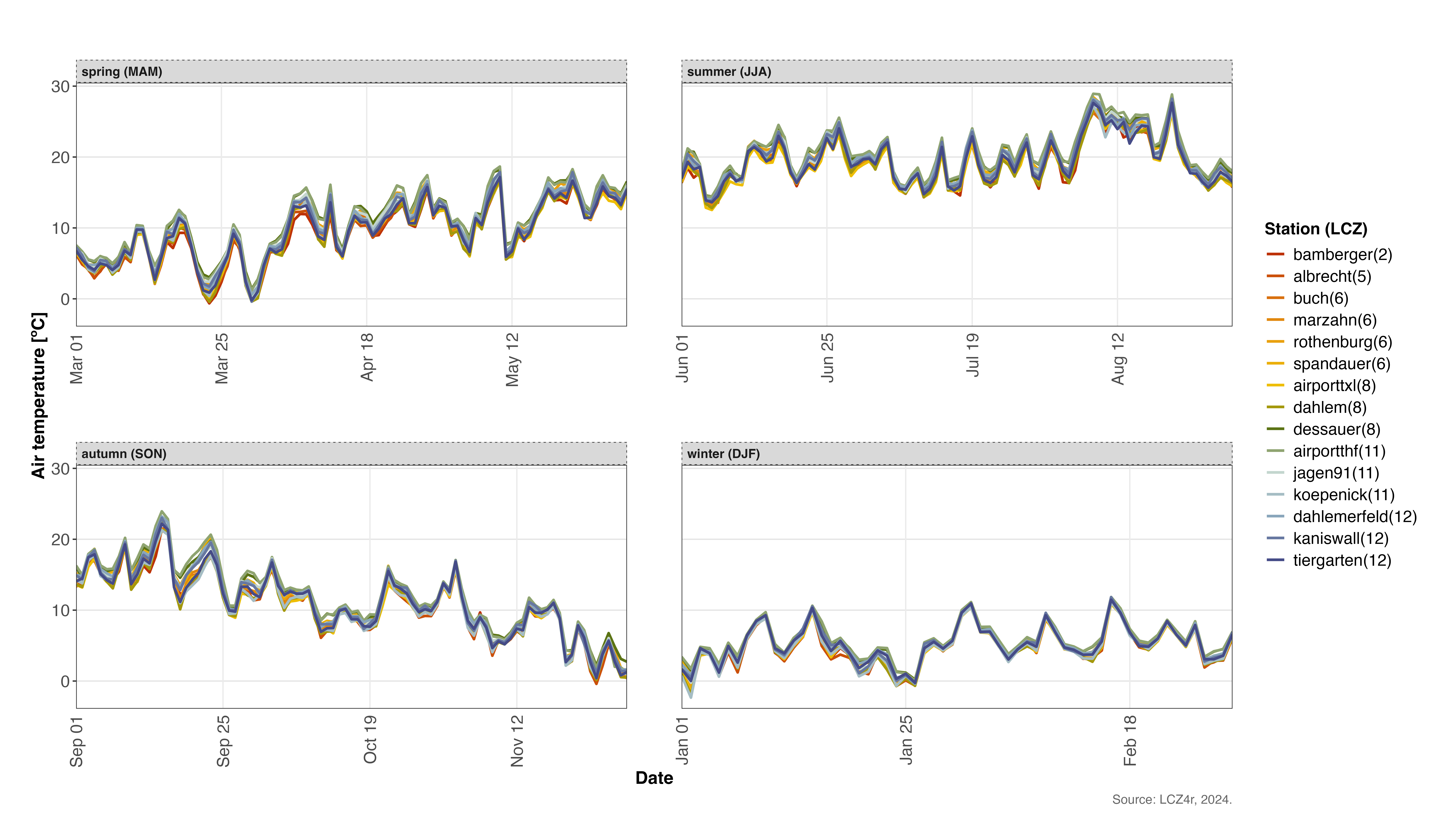
Splitting Data with the “by” argument

You can split data by temporal or spatial categories such as “year”, “month”, “season”, “weekday”, “weekend”, “yearseason”, and more.

#Daily air temperature by seasons of 2020
lcz_ts(lcz_map, data_frame = lcz_data, var = "airT", 
       station_id = "station", time.freq = "day",
       year = 2020,
       plot_type = "basic_line", 
       by="season"
       )

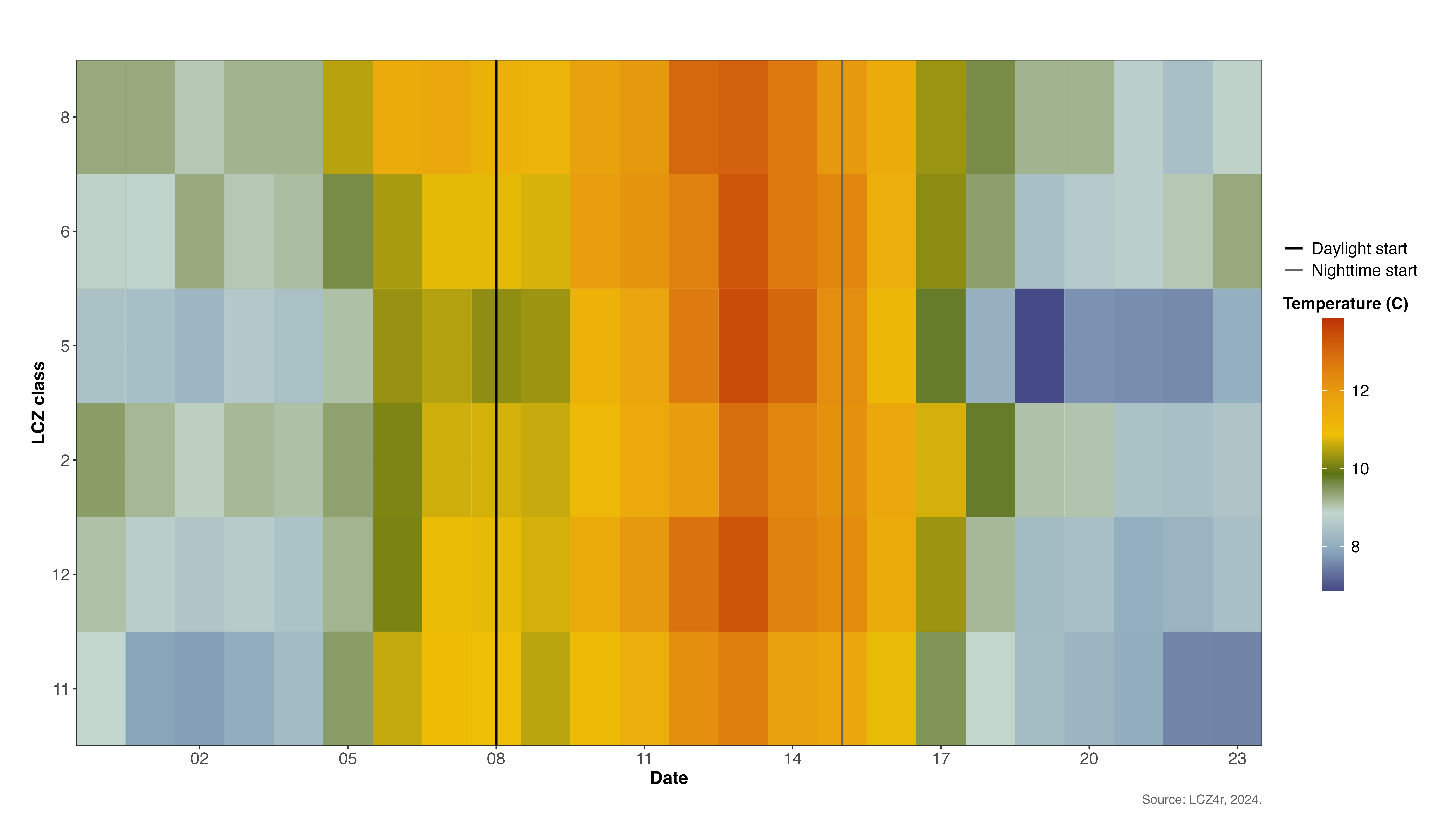
Dividing nighttime and daytime with “by” argument

You can also split data by nighttime and daytime periods with by=“daylight”.

#Diurnal cycle of air temperature on 15th January of 2020
lcz_ts(lcz_map, data_frame = lcz_data, var = "airT", 
       station_id = "station", time.freq = "hour",
       year = 2020, month=1, day=15
       plot_type = "heatmap", 
       by="daylight"
       )

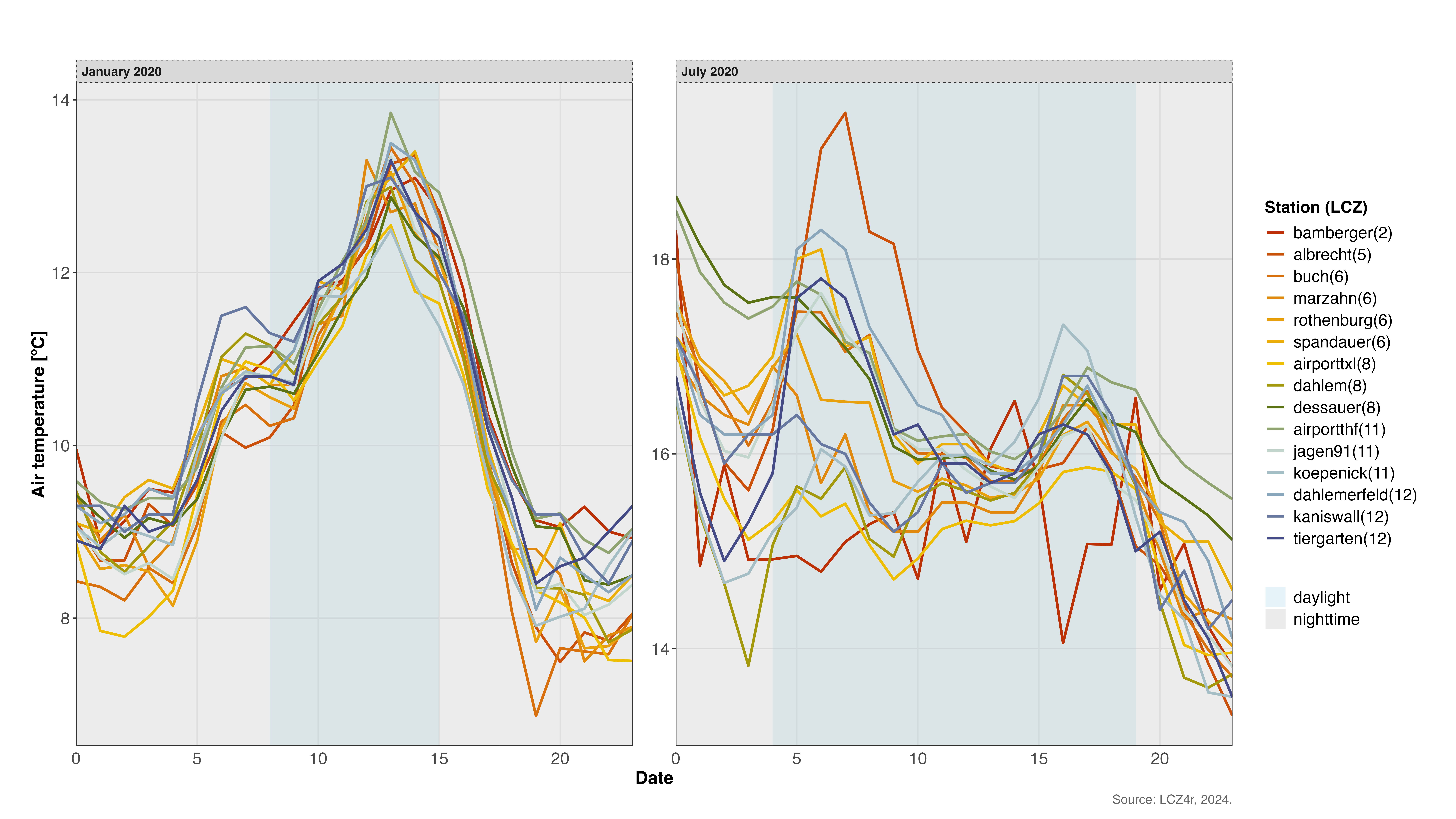
Combining daylight with months

#Diurnal cycle of air temperature on 15th January and July of 2020
lcz_ts(lcz_map, data_frame = lcz_data, var = "airT", 
       station_id = "station", time.freq = "hour",
       year = 2020, month=c(1, 7), day=15
       plot_type = "basic_line", 
       by= c("daylight", "monthyear")
       )

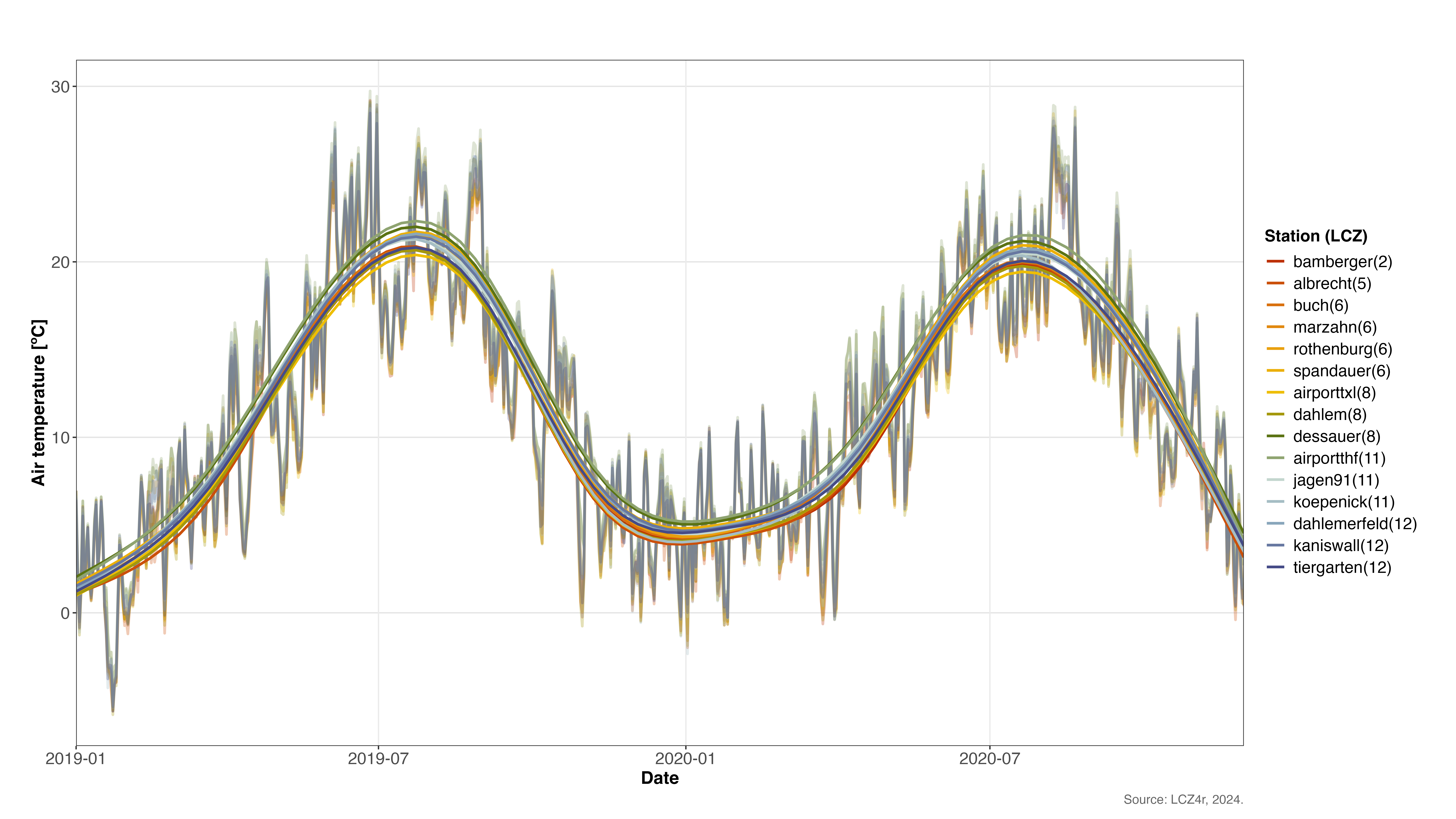
Smoothing Temperature Trends

Enable smoothing by setting smooth = TRUE, which adds a generalized additive model (GAM) line to show the temperature trend.


#Tends of daily air temperature for 2019 and 2020 by station
lcz_ts(lcz_map, data_frame = lcz_data, var = "airT", 
       station_id = "station", time.freq = "hour",
       year = 2019:2020,
       plot_type = "basic_line", 
       smooth= TRUE
       )

Save plots

To save a plot and dataframe, set isave = TRUE and specify the file type with save_extension (e.g., “png”,“jpeg”, “svg”, and “pdf”). A folder LCZ4r_output is created into PC.

#Save daylight plot and dataframe into PC
lcz_ts(lcz_map, data_frame = lcz_data, var = "airT", 
       station_id = "station", time.freq = "hour",
       year = 2020, month=1, day=15
       plot_type = "basic_line", by="daylight", 
       isave=TRUE
       )

Return a dataframe as result

To save return in R, set iplot = FALSE and create an object.

#Return daylight dataframe on 15th January of 2020
my_output <- lcz_ts(lcz_map, data_frame = lcz_data, var = "airT", 
       station_id = "station", time.freq = "hour",
       year = 2020, month=1, day=15
       plot_type = "basic_line", by="daylight", 
       iplot=FALSE
       )

Have feedback or suggestions?

Do you have an idea for improvement or did you spot a mistake? We’d love to hear from you! Click the button below to create a new issue (Github) and share your feedback or suggestions directly with us.

Max Anjos

November 11, 2024