Urban Heat Island (UHI) Analysis

Max Anjos

March 25, 2026

Introduction

The lcz_uhi_intensity() function is designed to calculate the Urban Heat Island (UHI) intensity based on air temperature measurements and Local Climate Zones (LCZ). UHI intensity is defined as the temperature difference between urban and rural areas, providing a quantitative measure of how much warmer urban areas are compared to their surrounding rural environments.

This guide demonstrates how to use the lcz_uhi_intensity() function to calculate and analyze UHI intensity using LCZ classes. The function supports two calculation methods:

Method 1: LCZ-Based Method

Automatically identifies LCZ built types (LCZ 1-10) to represent urban temperature, while LCZ natural types (LCZ A-G / 11-17) represent rural temperature. This method is ideal when you have comprehensive LCZ classification across your study area.

Method 2: Manual Method

Allows users to manually select specific stations as references for urban and rural areas. This method is useful when you have pre-defined reference stations or when LCZ classification is incomplete.

library(LCZ4r)

# Get the LCZ map for your city
lcz_map <- lcz_get_map_euro(city = "Berlin")

# Load sample data from LCZ4r
data("lcz_data")

Understanding UHI Intensity:

• Positive UHI intensity (red): Urban areas are warmer than rural areas (typical urban heat island)
• Negative UHI intensity (blue): Urban areas are cooler than rural areas (urban cool island)
• Zero UHI intensity: No temperature difference between urban and rural areas

UHI intensity typically peaks during nighttime and can vary significantly by season and weather conditions.

UHI Time Series

This example calculates hourly UHI intensity aggregated by month for the year 2019, providing insights into seasonal patterns of urban heating.

# Calculate hourly UHI intensity by month for 2019
lcz_uhi_intensity(lcz_map, 
                  data_frame = lcz_data, 
                  var = "airT", 
                  station_id = "station",
                  time.freq = "hour", 
                  method = "LCZ",
                  year = 2019,
                  by = "month")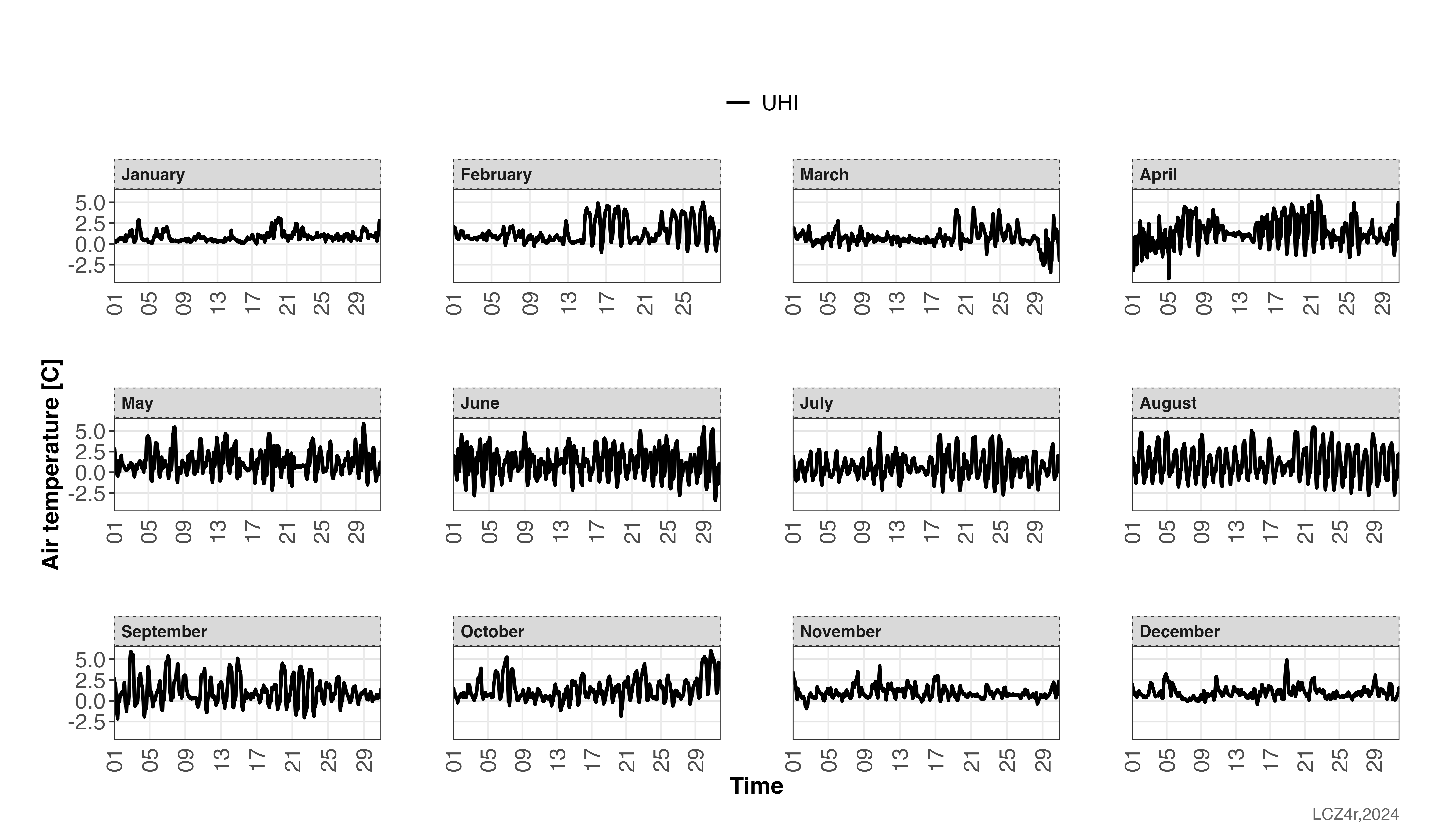

Monthly UHI intensity time series for Berlin in 2019. Positive values indicate urban areas are warmer than rural areas, with peak intensity typically observed during summer months.

UHI Seasonality

This analysis splits the data by season, providing a more detailed view of how UHI intensity varies throughout the year. The group = TRUE parameter also displays the urban and rural temperature components separately.

# Calculate hourly UHI intensity by season for 2019, including urban and rural temperatures
lcz_uhi_intensity(lcz_map, 
                  data_frame = lcz_data, 
                  var = "airT", 
                  station_id = "station",
                  time.freq = "hour", 
                  method = "LCZ",
                  year = 2019,
                  by = "season",
                  group = TRUE)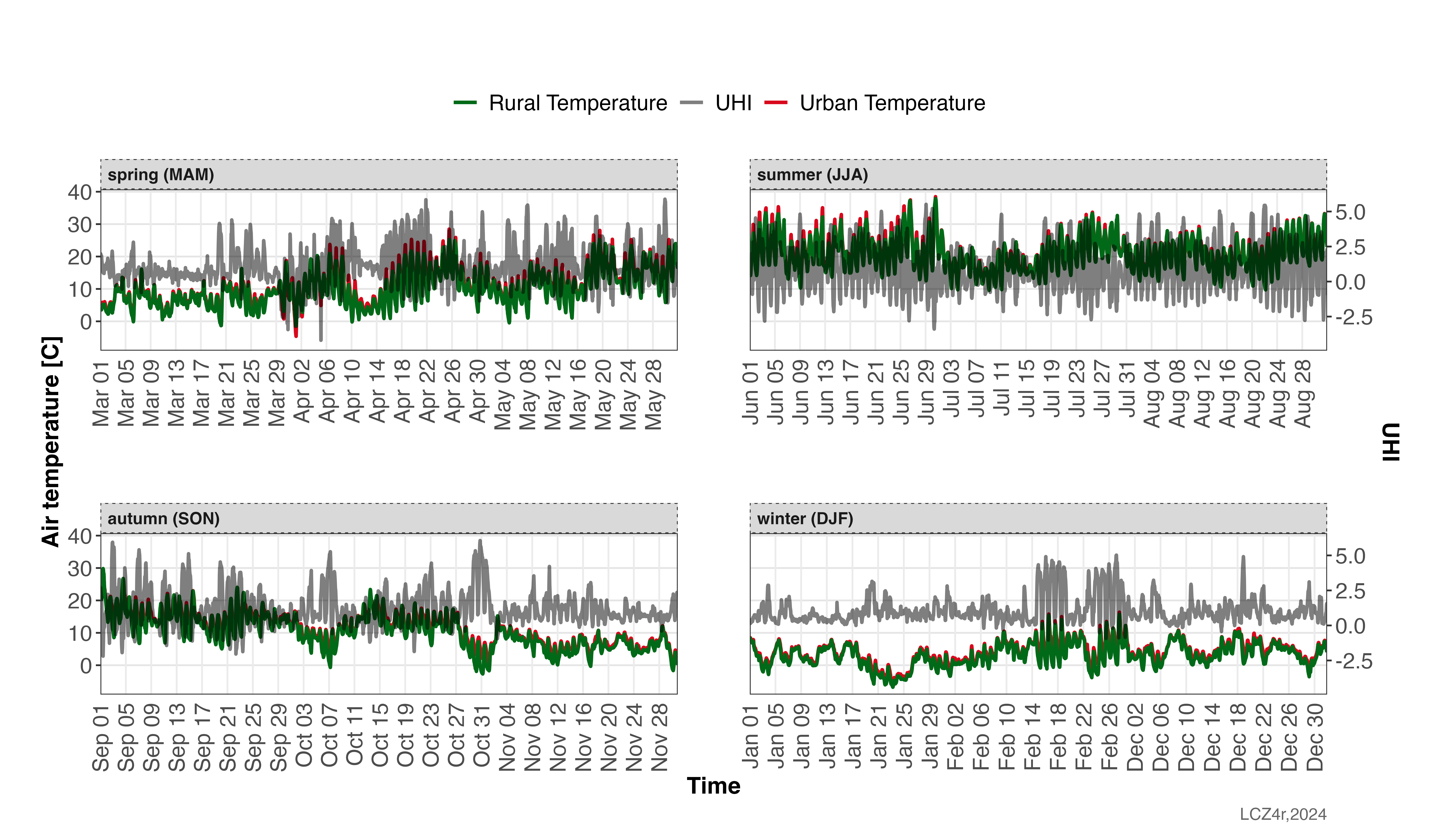

Seasonal UHI intensity patterns showing urban and rural temperature components. This visualization helps identify seasonal variations in UHI magnitude and the contributing temperature differences.

UHI Diurnal Cycle

Understanding the diurnal (day-night) cycle of UHI intensity is crucial for urban climate studies. This example calculates the diurnal pattern for a specific date.

# Calculate diurnal cycle of UHI intensity for February 6, 2019
lcz_uhi_intensity(lcz_map, 
                  data_frame = lcz_data, 
                  var = "airT", 
                  station_id = "station",
                  time.freq = "hour", 
                  method = "LCZ",
                  year = 2019, month = 2, day = 6,
                  by = "daylight",
                  group = TRUE)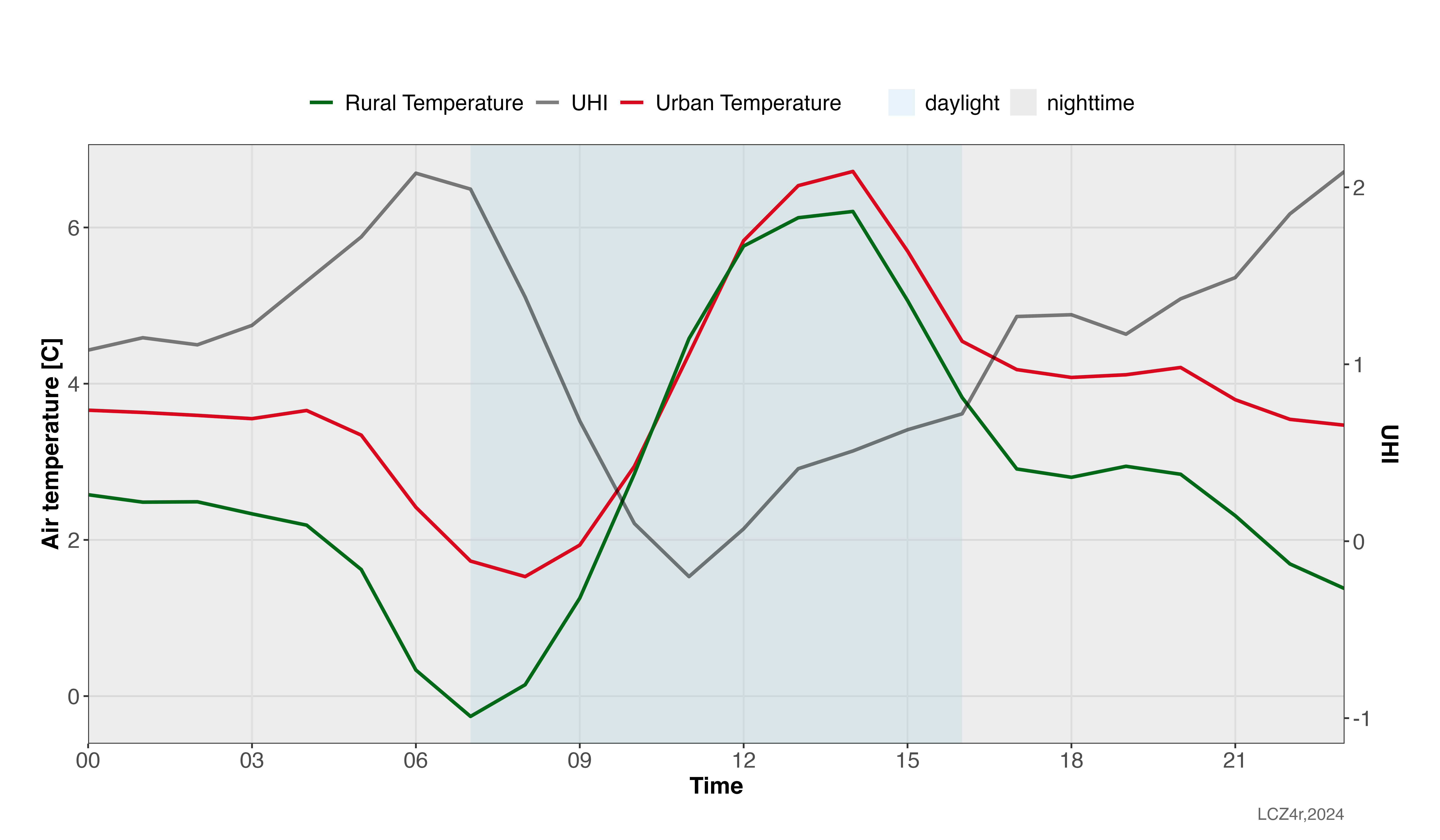

Diurnal cycle of UHI intensity on February 6, 2019, showing distinct patterns between daytime and nighttime periods. UHI intensity typically strengthens after sunset.

Manual Method: Custom Reference Selection

The manual method allows you to specify custom stations as urban and rural references. This is particularly useful when you have specific monitoring stations that serve as representative references for your study area.

# Calculate diurnal cycle of UHI intensity for February and July 2019 using manual method
lcz_uhi_intensity(lcz_map, 
                  data_frame = lcz_data, 
                  var = "airT", 
                  station_id = "station",
                  time.freq = "hour", 
                  year = 2019, month = c(2, 7), day = 6,
                  method = "manual",
                  Turban = "bamberger",      # Urban reference station
                  Trural = "airporttxl",     # Rural reference station
                  by = c("daylight", "month"),
                  group = TRUE)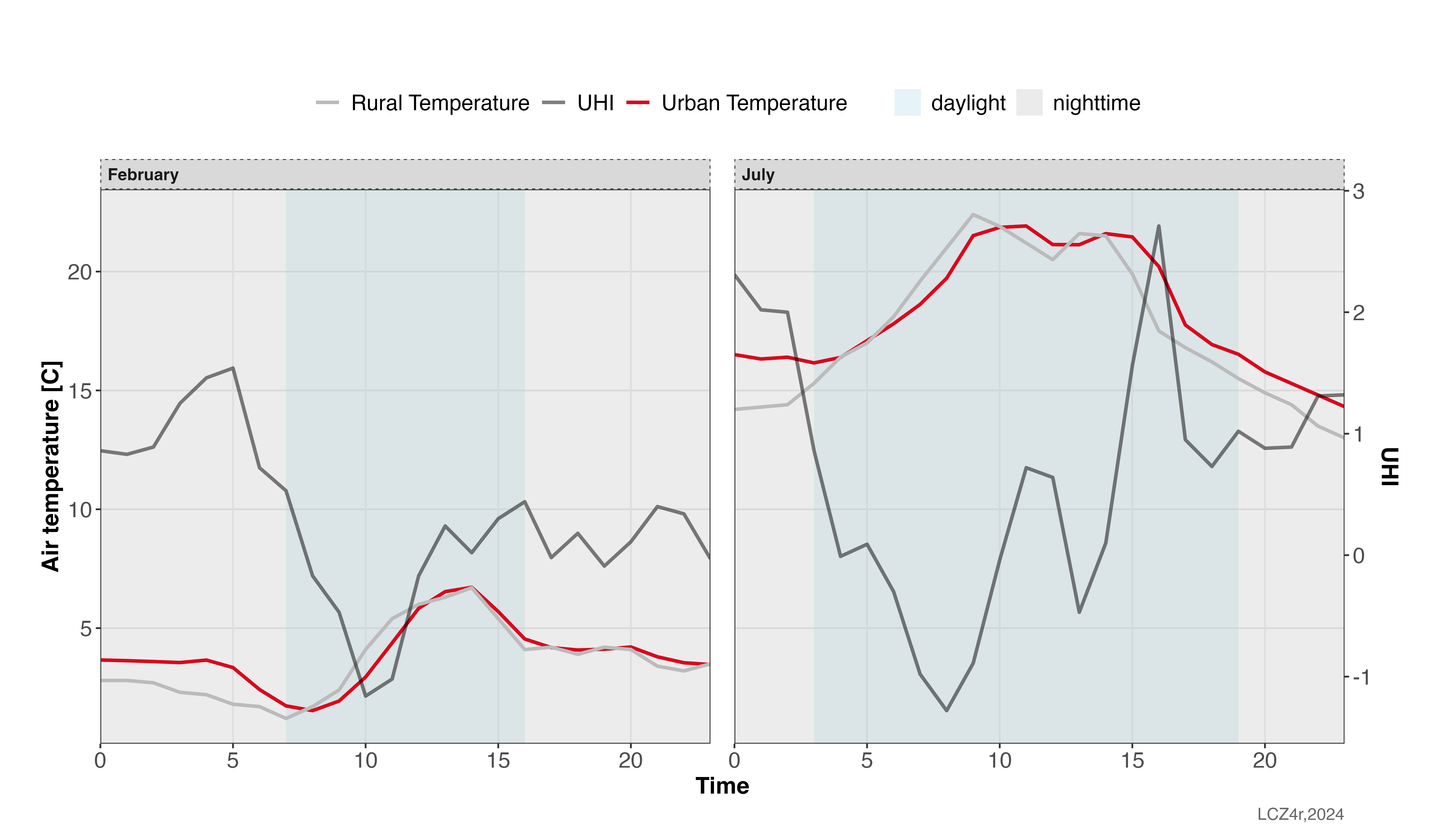

UHI intensity comparison between winter (February) and summer (July) 2019 using custom reference stations. This demonstrates the flexibility of the manual method for targeted analysis.

Advanced Analysis Options

Multiple Time Frequencies

You can analyze UHI intensity at different temporal aggregations:

# Daily UHI intensity for summer 2019
daily_uhi <- lcz_uhi_intensity(lcz_map, 
                               data_frame = lcz_data, 
                               var = "airT", 
                               station_id = "station",
                               time.freq = "day", 
                               method = "LCZ",
                               year = 2019, month = 6:8,
                               iplot = FALSE)

# Monthly UHI intensity for 2019
monthly_uhi <- lcz_uhi_intensity(lcz_map, 
                                 data_frame = lcz_data, 
                                 var = "airT", 
                                 station_id = "station",
                                 time.freq = "month", 
                                 method = "LCZ",
                                 year = 2019,
                                 iplot = FALSE)

Combining Multiple Splitting Options

You can combine multiple splitting criteria for more detailed analysis:

# UHI intensity by weekday and season
lcz_uhi_intensity(lcz_map, 
                  data_frame = lcz_data, 
                  var = "airT", 
                  station_id = "station",
                  time.freq = "hour", 
                  method = "LCZ",
                  year = 2019,
                  by = c("weekday", "season"),
                  group = TRUE)

Statistical Summary

You can return the data frame for further statistical analysis:

# Return UHI intensity data frame for statistical analysis
uhi_data <- lcz_uhi_intensity(lcz_map, 
                              data_frame = lcz_data, 
                              var = "airT", 
                              station_id = "station",
                              time.freq = "hour", 
                              method = "LCZ",
                              year = 2019,
                              iplot = FALSE)

# Calculate summary statistics
summary(uhi_data)

# Calculate seasonal means
aggregate(uhi_value ~ season, data = uhi_data, FUN = mean)

Save Plots

To save plots to your computer, set isave = TRUE and specify the file type:

# Save UHI intensity plot to PC
lcz_uhi_intensity(lcz_map, 
                  data_frame = lcz_data, 
                  var = "airT", 
                  station_id = "station",
                  time.freq = "hour", 
                  method = "LCZ",
                  year = 2019,
                  by = "season",
                  group = TRUE,
                  isave = TRUE,
                  save_extension = "png")

Tip: Saved plots are automatically organized in the LCZ4r_output folder with descriptive filenames including the analysis parameters and timestamp.

Practical Applications of UHI Analysis

Understanding UHI intensity patterns can inform various urban planning and climate adaptation strategies:

1. Heatwave Preparedness

Identify periods and areas with highest UHI intensity to target heatwave interventions and early warning systems.

2. Urban Planning

Use seasonal and diurnal patterns to guide urban design decisions, such as: - Placement of green infrastructure - Building height and density regulations - Cool material implementation strategies

3. Climate Change Adaptation

Establish baseline UHI patterns to monitor changes over time and evaluate the effectiveness of mitigation measures.

4. Public Health Planning

Identify vulnerable populations in areas with persistent high UHI intensity for targeted health interventions.

Important Considerations:

• UHI intensity calculations require adequate spatial coverage of monitoring stations across both urban and rural areas
• Weather conditions (wind speed, cloud cover) can significantly influence UHI intensity
• The LCZ method assumes that built LCZs represent urban conditions and natural LCZs represent rural conditions
• Consider using the manual method when LCZ classification is incomplete or when specific reference stations are preferred

Summary of Parameters

Here’s a quick reference for the main parameters used in lcz_uhi_intensity():

Parameter	Description	Options
time.freq	Temporal aggregation frequency	“hour”, “day”, “month”, “year”
method	Calculation method	“LCZ” (automatic), “manual” (custom)
Turban	Urban reference station (manual method)	Station ID for urban reference
Trural	Rural reference station (manual method)	Station ID for rural reference
by	Data splitting method	“month”, “season”, “daylight”, “weekday”, etc.
group	Display urban/rural components	TRUE/FALSE
isave	Save output to PC	TRUE/FALSE
iplot	Display plot	TRUE/FALSE

Interpreting Results

When analyzing UHI intensity results, consider:

• Peak intensity times: Typically 3-5 hours after sunset
• Seasonal patterns: Often strongest in summer and winter (depending on climate)
• Weather influences: Clear, calm nights produce strongest UHI signals
• Urban morphology: Compact built areas usually show higher intensity than open areas
• Vegetation effects: Green spaces can significantly reduce local UHI intensity

---

Have feedback or suggestions?

Do you have an idea for improvement or did you spot a mistake? We’d love to hear from you! Click the button below to create a new issue (GitHub) and share your feedback or suggestions directly with us.

Open GitHub issue