入门
热异常是评估城市内气温差异的好方法。在每个 LCZ 站,热异常定义为其温度与所有 LCZ 站的总体平均温度之间的差异。例如,正温度异常表明特定 LCZ 比所有其他 LCZ 更温暖。
这 lcz_anomaly() 函数具有与 lcz_ts()
关于时间选择的灵活性和通过时间窗口或站点分割
LCZ 时间序列。
library(LCZ4r)

# 获取您所在城市的LCZ地图
lcz_map <- lcz_get_map_euro(city = "Berlin")

# 从LCZ4r加载样本数据
data("lcz_data")了解热异常:
- 正异常(红色/暖色):车站温度高于城市平均水平
- 负异常(蓝色/冷色):车站比城市平均温度凉爽
- 零异常:站点温度等于城市平均值
该指标有助于识别城市内的城市热岛和凉爽点。
使用plot_type 绘制选项
这 plot_type 论证中 lcz_anomaly()
提供多种可视化效果:
- “diverging_bar”:从中心(零)发散的水平条形图,正异常向右延伸,负异常向左延伸
- “条形”:显示每个站点的异常幅度的条形图,根据异常是正还是负来着色
- “dot”:显示平均温度值和参考值的点图,并用线连接它们
- “棒棒糖”:棒棒糖图,其中每个“棒”代表一个异常值,顶部的点代表异常的大小
以下是使用每种绘图类型的示例。
1. 发散条形图
# 2019年2月6日05:00的热异常情况
lcz_anomaly(lcz_map,
            data_frame = lcz_data,
            var = "airT",
            station_id = "station",
            time.freq = "hour",
            year = 2019, month = 2, day = 6, hour = 5,
            plot_type = "diverging_bar",
            ylab = "Air temperature [°C]",
            xlab = "Stations",
            title = "LCZ Thermal Anomalies",
            caption = "Source: LCZ4r, 2024")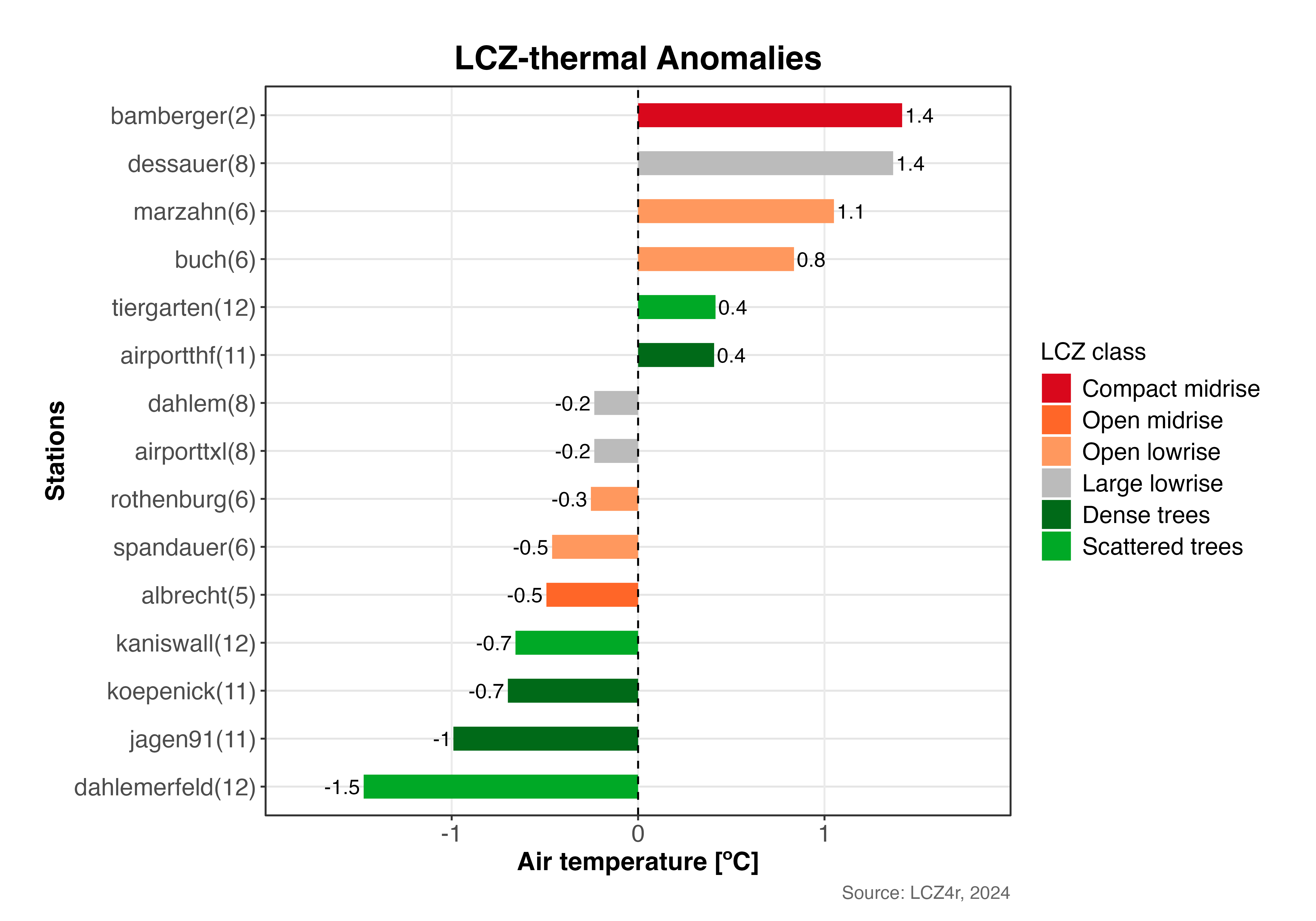
显示柏林 LCZ 站热异常的发散条形图(2019 年 2 月 6 日 05:00)。正异常(红色)表示较温暖的站点,负异常(蓝色)表示较冷的站点。
2. 条形图
# 2019年2月6日05:00的柱状图
lcz_anomaly(lcz_map,
            data_frame = lcz_data,
            var = "airT",
            station_id = "station",
            time.freq = "hour",
            year = 2019, month = 2, day = 6, hour = 5,
            plot_type = "bar")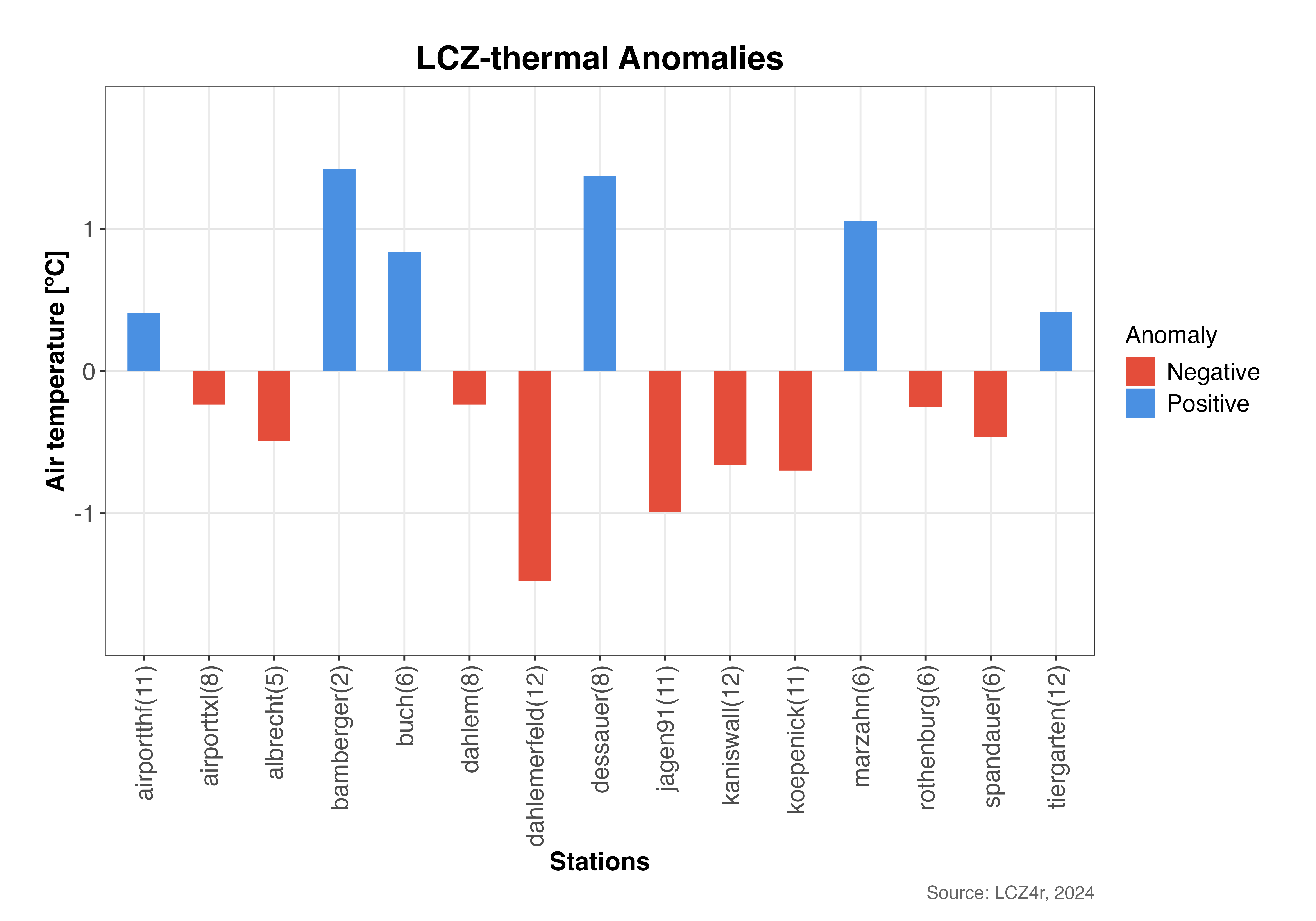
显示每个站热异常强度的条形图。延伸到零以上的条形表示正异常(较暖),低于零的条形表示负异常(较冷)。
3. 点图
# 2019年2月6日05:00的点阵图
lcz_anomaly(lcz_map,
            data_frame = lcz_data,
            var = "airT",
            station_id = "station",
            time.freq = "hour",
            year = 2019, month = 2, day = 6, hour = 5,
            plot_type = "dot")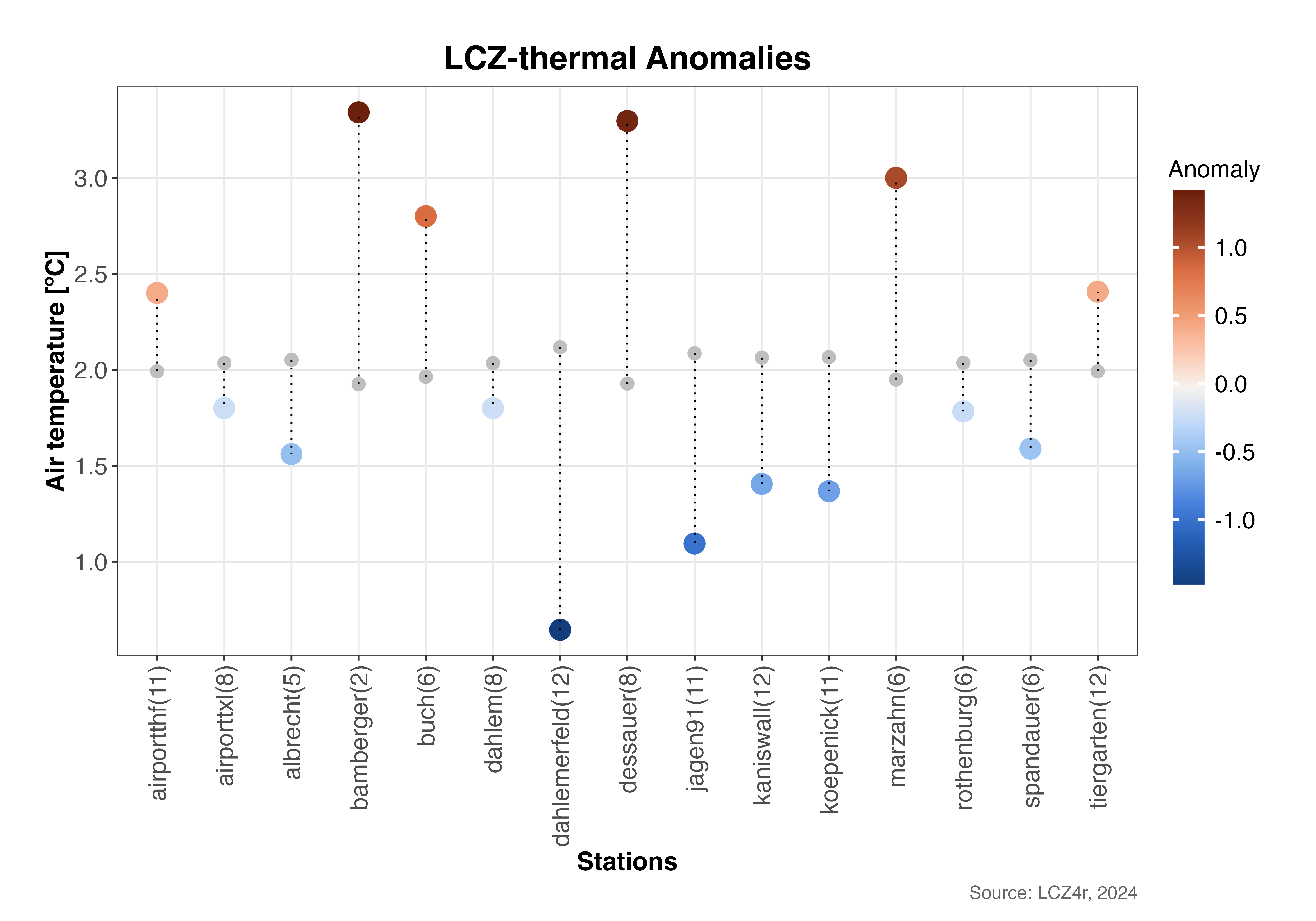
点图显示各个站点温度(彩色点)与城市平均温度(垂直虚线)的比较。距线的距离代表热异常幅度。
4. 棒棒糖情节
# 2019年2月6日05:00的棒棒糖图
lcz_anomaly(lcz_map,
            data_frame = lcz_data,
            var = "airT",
            station_id = "station",
            time.freq = "hour",
            year = 2019, month = 2, day = 6, hour = 5,
            plot_type = "lollipop")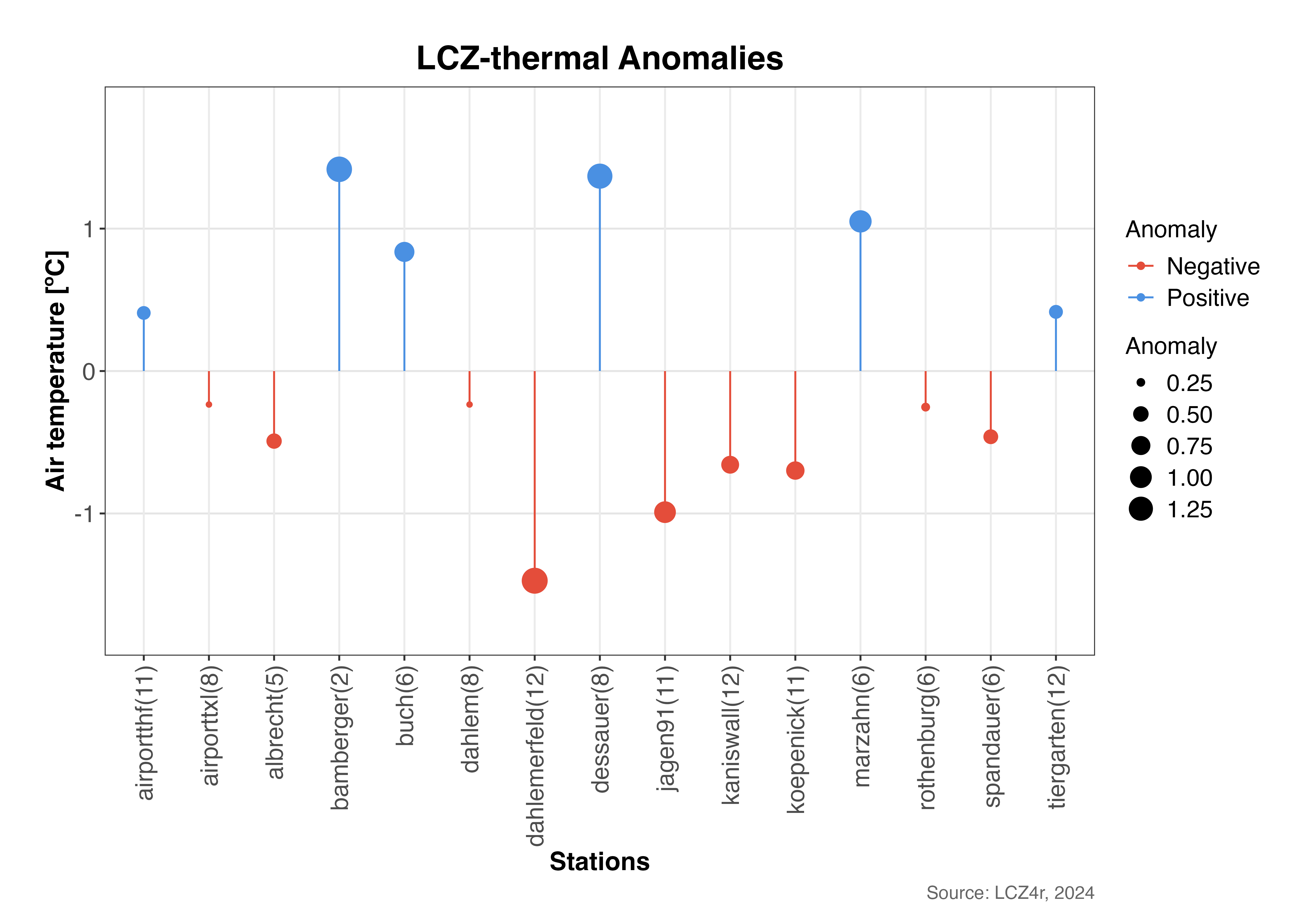
棒棒糖图强调热异常的大小和方向。每根“棒”的长度代表异常值,点的大小表示异常值的大小。
使用“by”参数分割异常
白天与夜间比较
# 计算2019年2月6日夜间和白天的异常值
lcz_anomaly(lcz_map,
            data_frame = lcz_data,
            var = "airT",
            station_id = "station",
            time.freq = "hour",
            year = 2019, month = 2, day = 6,
            plot_type = "diverging_bar",
            by = "daylight")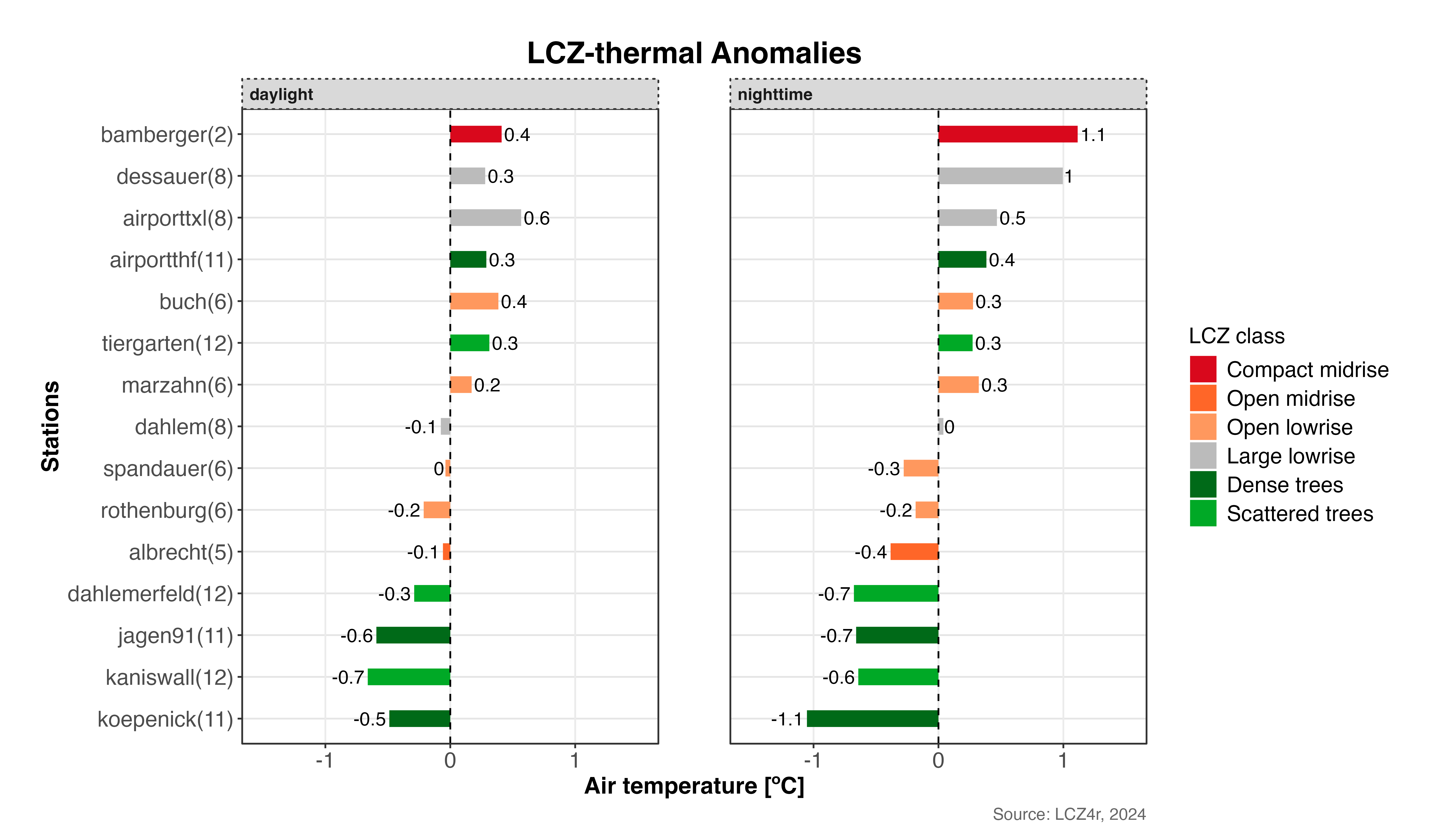
2019 年 2 月 6 日白天和夜间的热异常比较。这揭示了城市热模式在昼夜期间的变化。
将日光与月份结合起来
# 计算2019年2月和8月的月平均异常值
lcz_anomaly(lcz_map,
            data_frame = lcz_data,
            var = "airT",
            station_id = "station",
            time.freq = "hour",
            year = 2019, month = c(2, 8),
            plot_type = "bar",
            by = c("daylight", "month"))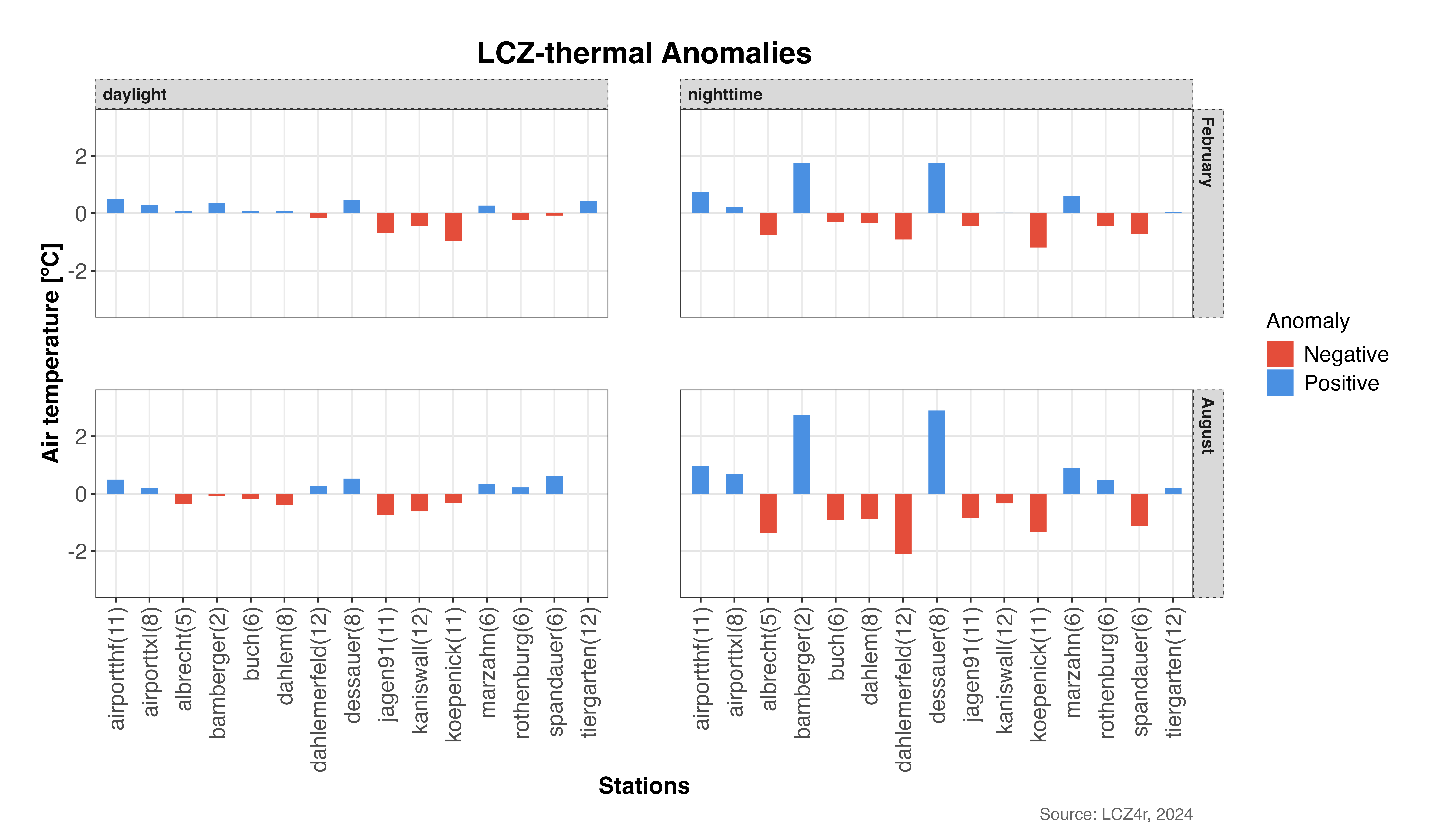
热异常的季节和昼夜模式:比较冬季(二月)和夏季(八月)的白天和夜间。
高级分析选项
时间聚合
您可以聚合不同时间频率的异常:
# 计算2019年2月的每日平均异常值
daily_anomalies <- lcz_anomaly(lcz_map,
                               data_frame = lcz_data,
                               var = "airT",
                               station_id = "station",
                               time.freq = "day",
                               year = 2019, month = 2,
                               plot_type = "bar",
                               iplot = FALSE)

# 计算 2019 年的月平均异常值
monthly_anomalies <- lcz_anomaly(lcz_map,
                                 data_frame = lcz_data,
                                 var = "airT",
                                 station_id = "station",
                                 time.freq = "month",
                                 year = 2019,
                                 plot_type = "bar",
                                 iplot = FALSE)
自定义视觉外观
# 自定义发散柱状图,可添加特定颜色和标签
lcz_anomaly(lcz_map,
            data_frame = lcz_data,
            var = "airT",
            station_id = "station",
            time.freq = "hour",
            year = 2019, month = 7, day = 15, hour = 14,  # Summer afternoon
            plot_type = "diverging_bar",
            ylab = "Temperature Anomaly [°C]",
            xlab = "LCZ Classes",
            title = "Summer Afternoon Thermal Anomalies",
            subtitle = "July 15, 2019 - 14:00h",
            caption = "Source: LCZ4r, 2024")
返回数据框作为结果
要将结果保存在 R 中,请设置 iplot = FALSE
并创建一个对象。
# 返回包含 2019 年 2 月和 8 月热异常数据的数据框
my_output <- lcz_anomaly(lcz_map,
                         data_frame = lcz_data,
                         var = "airT",
                         station_id = "station",
                         time.freq = "hour",
                         year = 2019, month = c(2, 8),
                         plot_type = "bar",
                         by = c("daylight", "month"),
                         iplot = FALSE)

# 查看返回的数据框的结构
str(my_output)

# 查看前几行
head(my_output)
保存地块
要将绘图保存到计算机,请设置 isave = TRUE 并指定文件类型
save_extension (例如,“png”、“jpeg”、“svg”、“pdf”)。
# 将热异常图保存到电脑
lcz_anomaly(lcz_map,
            data_frame = lcz_data,
            var = "airT",
            station_id = "station",
            time.freq = "hour",
            year = 2019, month = 7, day = 15, hour = 14,
            plot_type = "diverging_bar",
            by = "daylight",
            isave = TRUE,
save_extension = "png")提示:保存的图将自动组织在 LCZ4r_output
带有时间戳的文件名的文件夹,以便于参考。该文件夹将在您当前的工作目录中创建。
参数汇总
以下是主要参数的快速参考 lcz_anomaly():
| 参数 | 描述 | 选项 |
|---|---|---|
time.freq |
时间聚合频率 | “时”、“日”、“月”、“年” |
plot_type |
可视化类型 | “diverging_bar”、“bar”、“dot”、“棒棒糖” |
by |
数据分割方式 | “日光”、“月份”、“季节”、“工作日”等 |
isave |
将输出保存到 PC | 对/错 |
iplot |
显示图 | 对/错 |
var |
要分析的变量 | 带有温度数据的列名称 |
station_id |
站标识符栏 | 带有站 ID 的列名称 |